
视觉伺服入门第三步:智能机器人控制论文阅读 Dealing with constraints in sensor-based robot control
想要更好的食用,建议先品尝如下两篇论文视觉伺服入门第一步:带你从经典论文阅读Visual servo control. I. Basic approach开启视觉伺服之旅视觉伺服入门第二步:带你从经典论文阅读Visual Servo Control Part II: Advanced Approaches进阶版论文摘要在本文中提出了一个多传感器机器人在多种约束条件下的控制框架。我们将来自多个传感器
想要更好的食用,建议先品尝如下两篇论文
- 视觉伺服入门第一步:带你从经典论文阅读Visual servo control. I. Basic approach开启视觉伺服之旅
- 视觉伺服入门第二步:带你从经典论文阅读Visual Servo Control Part II: Advanced Approaches进阶版
论文摘要
在本文中提出了一个多传感器机器人在多种约束条件下的控制框架。我们将来自多个传感器的特征处理为单个特征向量。我们方法的核心思想是考虑所有的约束因素,利用加权矩阵平衡每个特性的贡献。约束的添加使得我们的控制环节更加平滑。在控制设计中引入了多传感器建模的这一方法与线性二次控制相似。本篇论文主要讲述 的是三维定位6自由度机械臂的视觉伺服。任务要确保多个约束组合的同时执行。
我们所考虑的约束条件有可视性以及关节限制规避等。
A framework is presented in this paper for the control of a multi-sensor robot under several constraints. In this approach, the features coming from several sensors are treated as a single feature vector. The core of our approach is a weighting matrix that balances the contribution of each feature, allowing to take constraints into account.
多传感器建模
This section presents the general modeling of a multi-sensor robot. First, we define the global kinematic model, then we introduce the weighted signal error that will be used in the control law. We propose a generic weighting function that allows both balancing the sensor features and taking into account unilateral constraints.

我们之前已经推导过了特征雅克比的公式。
s ˙ = L s c W e J ( q ) q ˙ \dot \mathbf{s}=\mathbf{L_s}{}^c\mathbf{W}_e\mathbf{J}(q)\dot q s˙=LscWeJ(q)q˙
多传感器的测量向量为 s = ( s 1 , s 2 , s 3 , s 4 . . . , s k ) \mathbf{s}=(\mathbf{s}_1,\mathbf{s}_2,\mathbf{s}_3,\mathbf{s}_4...,\mathbf{s}_k) s=(s1,s2,s3,s4...,sk),每一个测量的维度为m。我们可以得到如下运动学模型。
J s = L W e J q = [ L 1 … 0 ⋮ ⋱ ⋮ 0 … L k ] [ 1 W e ⋮ k W e ] e J q \mathbf{J}_{s}=\mathbf{L W}_{e}{\mathbf{J}}_{q}=\left[\begin{array}{ccc} \mathbf{L}_{1} & \ldots & 0 \\ \vdots & \ddots & \vdots \\ 0 & \ldots & \mathbf{L}_{k} \end{array}\right]\left[\begin{array}{c} { }^{1} \mathbf{W}_{e} \\ \vdots \\ { }^{k} \mathbf{W}_{e} \end{array}\right]{}^{e} \mathbf{J}_{q} Js=LWeJq=⎣⎢⎡L1⋮0…⋱…0⋮Lk⎦⎥⎤⎣⎢⎡1We⋮kWe⎦⎥⎤eJq
此外,我们需要设置每一个任务的加权误差矩阵 e = H e ∗ e=\mathbf{H}e^* e=He∗:
H = [ H 1 … 0 ⋮ ⋱ ⋮ 0 … H k ] \mathbf{H}=\left[\begin{array}{ccc} \mathbf{H}_{1} & \ldots & 0 \\ \vdots & \ddots & \vdots \\ 0 & \ldots & \mathbf{H}_{k} \end{array}\right] H=⎣⎢⎡H1⋮0…⋱…0⋮Hk⎦⎥⎤
原始的control law为 e = s − s ∗ e=s-s^* e=s−s∗,换成关节空间
H J q ˙ = H ( s − s ∗ ) s . t . q ˙ = ( H J ) + H ( s − s ∗ ) \mathbf{H}\mathbf{J}\dot q=\mathbf{H}(s-s^*)\quad s.t. \quad \dot q=(\mathbf{H}\mathbf{J})^{+}\mathbf{H}(s-s^*) HJq˙=H(s−s∗)s.t.q˙=(HJ)+H(s−s∗)
我们的优化函数也在变 m i n ∣ ∣ J q ˙ − e ˙ ∗ ∣ ∣ 2 — — > m i n ∣ ∣ H J q ˙ − H e ˙ ∗ ∣ ∣ 2 min||\mathbf{J}\dot q-\dot e^*||^2——>min||\mathbf{H}\mathbf{J}\dot q-\mathbf{H}\dot e^*||^2 min∣∣Jq˙−e˙∗∣∣2——>min∣∣HJq˙−He˙∗∣∣2
∀ i ∈ [ 1 , m ] : h i = h i t + h i c \forall i \in[1, m]: h_{i}=h_{i}^{t}+h_{i}^{c} ∀i∈[1,m]:hi=hit+hic
我们一般考虑设置任务一定会用的特征,其加权 h i t = 1 h_{i}^{t}=1 hit=1;如果单纯考虑约束,我们把特征设置在 h i t = 0 h_{i}^{t}=0 hit=0;现在我们集中讨论的是 h i c h_{i}^{c} hic对于约束的影响。
例如下图,我们考虑的是图像坐标的约束, h i c h_{i}^{c} hic如何表达? 我们有安全区的存在。速写板
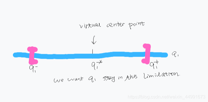
{ s i s − = s i − + ρ i ( s i + − s i − ) s i s + = s i + − ρ i ( s i + − s i − ) \left\{\begin{aligned} s_{i}^{\mathrm{s}-} &=s_{i}^{-}+\rho_{i}\left(s_{i}^{+}-s_{i}^{-}\right) \\ s_{i}^{\mathrm{s}+} &=s_{i}^{+}-\rho_{i}\left(s_{i}^{+}-s_{i}^{-}\right) \end{aligned}\right. {sis−sis+=si−+ρi(si+−si−)=si+−ρi(si+−si−)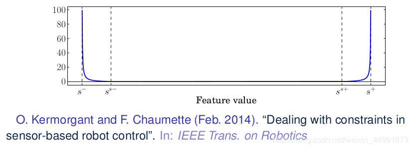
h i c = { s i − s i 8 + s i + − s i if s i > s i s + s i i − − s i s i − s i − if s i < s i s − 0 otherwise h_{i}^{c}=\left\{\begin{array}{cc} \frac{s_{i}-s_{i}^{8+}}{s_{i}^{+}-s_{i}} & \text { if } s_{i}>s_{i}^{\mathrm{s}+} \\ \frac{s_{i}^{i-}-s_{i}}{s_{i}-s_{i}^{-}} & \text {if } s_{i}<s_{i}^{\mathrm{s}-} \\ 0 & \text { otherwise } \end{array}\right. hic=⎩⎪⎪⎨⎪⎪⎧si+−sisi−si8+si−si−sii−−si0 if si>sis+if si<sis− otherwise
参考文献
[1] Olivier Kermorgant, François Chaumette. Dealing with constraints in sensor-based robot control.IEEE Transactions on Robotics, IEEE, 2014, 30 (1), pp.244-257. ff10.1109/TRO.2013.2281560ff. ffhal00855724f

一站式 AI 云服务平台
更多推荐


 0
0 0
0- 0


 已为社区贡献3条内容

所有评论(0)