python计算机视觉编程第五章多视图几何

多视图几何（Multiple View Geometry）是计算机视觉领域的一个重要概念，它涉及到从多个不同视角（角度）获取的图像中推断出物体的三维结构和相对位置关系。在现实世界中，我们通常通过不同的角度观察物体，然后通过这些不同的视角来理解物体的形状、位置和运动。多视图几何的目标就是从这些多个视图中恢复出物体的几何信息。主要内容有：三维重建、立体视觉、运动估计等。

m0_68784427

543人浏览 · 2023-08-14 21:34:24

m0_68784427 · 2023-08-14 21:34:24 发布

多视图几何

主要内容有：三维重建、立体视觉、运动估计等。

外极几何

外极几何是研究两幅图像之间存在的几何。它和场景结构无关，只依赖于摄像机的内外参数。

此处我们假设照相机的内参都标定过了，只有外参未知。为了方便，通常将外参的远点和坐标轴与第一个相机对齐，那么就有
$P_1 = K_1[I|0]和P_2 = K_2[R|t]$
其中 $K_1和K_2$ 是标定矩阵，是已知的。I和R分别是两个相机的旋转矩阵，t是第二个相机的平移量（因为我们认为第一个相机在原点，所以是0）。利用这些参数，我们就可以得到真实的点X的投影点， $x_1,x_2$ 的关系。也可以从 $x_1,x_2$ 反推这些参数。

同一个图像点经过不同的投影矩阵产生的不同投影点必须满足：
$x2TFx1=0\mathbf{x}_2^TF\mathbf{x}_1=0$
其中：
$F=K_2^{-T}S_tRK_1^{-1}$
矩阵 $S_t$ 为反对称矩阵：
$St=[0−t3t2t30−t1−t2t10]\boldsymbol{S}_\mathrm{t}=\begin{bmatrix}0&-t_3&t_2\\[0.3em]t_3&0&-t_1\\[0.3em]-t_2&t_1&0\end{bmatrix}$

由平移t组成。F称为基础矩阵，由于反对称矩阵行列式为0，故F的秩小于等于2。

我们可以借助F恢复照相机参数，F可以从对应的投影图像点计算X，K未知情况下，可以恢复出投影变换矩阵§，K已知，可以在三维重建中正确表示距离和角度。
$x_2^T Fx_1 = l_1^Tx_1=0$ ,找到第一幅图像的一条直线 $l_1^Tx_1=0$ ,第二个点在第一幅图像中的对应点一定在这条线（ $x_2$ 的外极线上），两条外极线都经过一个外极点e，是另一个照相机光心对应的图像点， $Fe_1 = e_2^tF = 0$ 。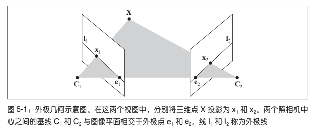
在这里插入图片描述

简单的数据集

我们先来读取一个简单的数据集：

from numpy import *
import scipy
from matplotlib import pyplot as plt
import cv2


class Camera(object):
    """ Class for representing pin-hole cameras. """
    
    def __init__(self,P):
        """ Initialize P = K[R|t] camera model. """
        self.P = P
        # 标定矩阵
        self.K = None # calibration matrix
        self.R = None # rotation
        self.t = None # translation
        # 照相机中心
        self.c = None # camera center
        
    
    def project(self,X):
        """    Project points in X (4*n array) and normalize coordinates. """
        
        #定义和坐标归一化 
        # (3,n)
        x = dot(self.P,X)
        for i in range(3):
            x[i] /= x[2]    
        return x
    def rotation_matrix(self,a):
        """    Creates a 3D rotation matrix for rotation
        around the axis of the vector a. """
        
        # 旋转矩阵
        R = eye(4)
        R[:3,:3] = scipy.linalg.expm([[0,-a[2],a[1]],[a[2],0,-a[0]],[-a[1],a[0],0]])
        return R
    
    def factor(self):
        """    Factorize the camera matrix into K,R,t as P = K[R|t]. """
        
        # 分解前三列
        K,R = scipy.linalg.rq(self.P[:,:3])
        # 分解后三列
        T = diag(sign(diag(K)))
        if linalg.det(T) < 0:
            T[1,1] *= -1
        self.K = dot(K,T)
        self.R = dot(T,R) # T is its own inverse
        self.t = dot(linalg.inv(self.K),self.P[:,3])
        
        return self.K, self.R, self.t
        
        
def my_calibration(sz):
    """
    Calibration function for the camera (iPhone4) used in this example.
    """
    row, col = sz
    fx = 2555*col/2592
    fy = 2586*row/1936
    K = diag([fx, fy, 1])
    K[0, 2] = 0.5*col
    K[1, 2] = 0.5*row
    return K

# 生成齐次坐标
def make_homog(points):
    """Convert points to homogeneous coordinates."""
    return vstack((points,ones((1,points.shape[1])))) 

def normalize(points):
    """ Normalize a collection of points in 
        homogeneous coordinates so that last row = 1. """

    for row in points:
        row /= points[-1]
    return points

from PIL import Image
from numpy import *
from pylab import *

# 载入一些图像
im1 = array(Image.open('images/001.jpg'))
im2 = array(Image.open('images/002.jpg'))
# 载入每个视图的二维点到列表中
points2D = [loadtxt('2D/00'+str(i+1)+'.corners').T for i in range(3)]
# 载入三维点
points3D = loadtxt('3D/p3d').T
# 载入对应
corr = genfromtxt('2D/nview-corners',dtype='int')
# 载入照相机矩阵到 Camera 对象列表中
P = [Camera(loadtxt('2D/00'+str(i+1)+'.P')) for i in range(3)]
# 将三维点转换成齐次坐标表示，并投影
X = vstack( (points3D,ones(points3D.shape[1])) )
x = P[0].project(X)
# 在视图 1 中绘制点
figure()
imshow(im1)
plot(points2D[0][0],points2D[0][1],'*')
axis('off')
figure()
imshow(im1)
plot(x[0],x[1],'r.')
axis('off')
show()

在这里插入图片描述

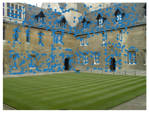
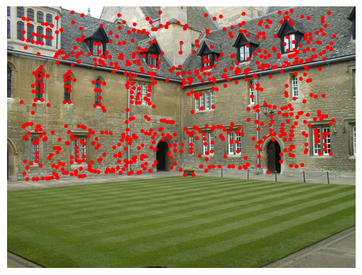
按照书上的说法，第二张图比第一张的点要多一些，多出来的点是从其他图片中重建出来的。我看了一会儿并没有发现有多很多点，猜测这可能是因为数据量太小的原因。

用Matplotlib绘制三维数据

使用下面的代码

from mpl_toolkits.mplot3d import axes3d
fig = figure()
ax = fig.add_subplot(projection='3d')
X,Y,Z = axes3d.get_test_data(0.25)
# 在三维中绘制点
ax.plot(X.flatten(),Y.flatten(),Z.flatten(),'o')
show()

即可得到下面的结果：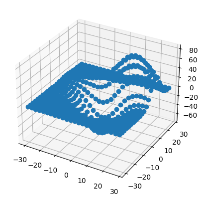
在这里插入图片描述
值得注意的是，书上的代码用的是fig.gca(projection=‘3d’)
，这个函数经我测试已经跑不通了，因此我改用了fig.add_subplot(projection=‘3d’)

计算F：八点法

八点法是通过对应点来计算基础矩阵的算法，外极约束可以写成线性系统的形式。
$[x21x11x21y11x21w11⋯w21w11x22x12x22y12x22w12⋯w22w12⋮⋮⋮⋱⋮x2nx1nx2ny1nx2nw1n⋯w2nw1n][F11F12F13⋮F33]=Af=0\begin{bmatrix}x_2^1x_1^1&x_2^1y_1^1&x_2^1w_1^1&\cdots&w_2^1w_1^1\\x_2^2x_1^2&x_2^2y_1^2&x_2^2w_1^2&\cdots&w_2^2w_1^2\\\vdots&\vdots&\vdots&\ddots&\vdots\\x_2^nx_1^n&x_2^ny_1^n&x_2^nw_1^n&\cdots&w_2^nw_1^n\end{bmatrix}\begin{bmatrix}F_{11}\\F_{12}\\F_{13}\\\vdots\\F_{33}\end{bmatrix}=A\boldsymbol{f}=0$
其中，f包含F的元素， $x_1^i和x_2^i$ 是一对图像点，共有n对对应点。基础矩阵中有 9 个元素，由于尺度是任意的，所以只需要 8 个方程。因为算法中需要 8 个对应点来计算基础矩阵 F，所以该算法叫做八点法。
八点法中最小化||Af||的函数：

def compute_fundamental(x1,x2):
    """ 使用归一化的八点算法，从对应点（x1，x2 3×n 的数组）中计算基础矩阵
    每行由如下构成：
    [x'*x，x'*y' x', y'*x, y'*y, y', x, y, 1]"""
    n = x1.shape[1]

    if x2.shape[1] != n:
        raise ValueError("Number of points don't match.")
    # 创建方程对应的矩阵
    A = zeros((n,9))
    for i in range(n):
        A[i] = [x1[0,i]*x2[0,i], x1[0,i]*x2[1,i], x1[0,i]*x2[2,i],
    x1[1,i]*x2[0,i], x1[1,i]*x2[1,i], x1[1,i]*x2[2,i],
    x1[2,i]*x2[0,i], x1[2,i]*x2[1,i], x1[2,i]*x2[2,i] ]
    # 计算线性最小二乘解
    U,S,V = linalg.svd(A)
    # V的最后一行有9个元素
    F = V[-1].reshape(3,3)
    # 受限 F
    # 通过将最后一个奇异值置 0，使秩为 2
    U,S,V = linalg.svd(F)
    S[2] = 0
    F = dot(U,dot(diag(S),V))
    return F

外极点和外极线

外极点们组 $Fe_1 = 0$ ，因此可以通过计算F的零空间来得到。

def compute_epipole(F):
 """ 从基础矩阵 F 中计算右极点（可以使用 F.T 获得左极点）"""
 # 返回 F 的零空间（Fx=0）
 U,S,V = linalg.svd(F)
 e = V[-1]
 # 归一化
 return e/e[2]

若想获得另一幅图像的外极点，只需将F转置后输入上述函数即可。

在Merton数据集的前两个视图上运行这两个函数：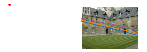
在这里插入图片描述

第一个视图画出了前5个外极线，第二个视图中画出了对应匹配点，可以看到，这些线在图片外左侧位置将相交于一点(就是那个红点，我给画出来了)。外极线上一定存在着另一个图像的对应点。
完整代码：

from numpy import *
import scipy
from matplotlib import pyplot as plt
import cv2


class Camera(object):
    """ Class for representing pin-hole cameras. """
    
    def __init__(self,P):
        """ Initialize P = K[R|t] camera model. """
        self.P = P
        # 标定矩阵
        self.K = None # calibration matrix
        self.R = None # rotation
        self.t = None # translation
        # 照相机中心
        self.c = None # camera center
        
    
    def project(self,X):
        """    Project points in X (4*n array) and normalize coordinates. """
        
        #定义和坐标归一化 
        # (3,n)
        x = dot(self.P,X)
        for i in range(3):
            x[i] /= x[2]    
        return x
    def rotation_matrix(self,a):
        """    Creates a 3D rotation matrix for rotation
        around the axis of the vector a. """
        
        # 旋转矩阵
        R = eye(4)
        R[:3,:3] = scipy.linalg.expm([[0,-a[2],a[1]],[a[2],0,-a[0]],[-a[1],a[0],0]])
        return R
    
    def factor(self):
        """    Factorize the camera matrix into K,R,t as P = K[R|t]. """
        
        # 分解前三列
        K,R = scipy.linalg.rq(self.P[:,:3])
        # 分解后三列
        T = diag(sign(diag(K)))
        if linalg.det(T) < 0:
            T[1,1] *= -1
        self.K = dot(K,T)
        self.R = dot(T,R) # T is its own inverse
        self.t = dot(linalg.inv(self.K),self.P[:,3])
        
        return self.K, self.R, self.t
        
        
def my_calibration(sz):
    """
    Calibration function for the camera (iPhone4) used in this example.
    """
    row, col = sz
    fx = 2555*col/2592
    fy = 2586*row/1936
    K = diag([fx, fy, 1])
    K[0, 2] = 0.5*col
    K[1, 2] = 0.5*row
    return K

# 生成齐次坐标
def make_homog(points):
    """Convert points to homogeneous coordinates."""
    return vstack((points,ones((1,points.shape[1])))) 

def normalize(points):
    """ Normalize a collection of points in 
        homogeneous coordinates so that last row = 1. """

    for row in points:
        row /= points[-1]
    return points


def compute_fundamental(x1,x2):
    """ 使用归一化的八点算法，从对应点（x1，x2 3×n 的数组）中计算基础矩阵
    每行由如下构成：
    [x'*x，x'*y' x', y'*x, y'*y, y', x, y, 1]"""
    n = x1.shape[1]

    if x2.shape[1] != n:
        raise ValueError("Number of points don't match.")
    # 创建方程对应的矩阵
    A = zeros((n,9))
    for i in range(n):
        A[i] = [x1[0,i]*x2[0,i], x1[0,i]*x2[1,i], x1[0,i]*x2[2,i],
    x1[1,i]*x2[0,i], x1[1,i]*x2[1,i], x1[1,i]*x2[2,i],
    x1[2,i]*x2[0,i], x1[2,i]*x2[1,i], x1[2,i]*x2[2,i] ]
    # 计算线性最小二乘解
    U,S,V = linalg.svd(A)
    # V的最后一行有9个元素
    F = V[-1].reshape(3,3)
    # 受限 F
    # 通过将最后一个奇异值置 0，使秩为 2
    U,S,V = linalg.svd(F)
    S[2] = 0
    F = dot(U,dot(diag(S),V))
    return F

def compute_epipole(F):
    """ 从基础矩阵 F 中计算右极点（可以使用 F.T 获得左极点）"""
    # 返回 F 的零空间（Fx=0）
    U,S,V = linalg.svd(F)
    e = V[-1]
    # 归一化
    return e/e[2]

def plot_epipolar_line(im,F,x,epipole=None,show_epipole=True):
    """ 在图像中，绘制外极点和外极线 F×x=0。F 是基础矩阵，x 是另一幅图像中的点 """
    m,n = im.shape[:2]
    line = dot(F,x)
    # 外极线参数和值
    t = linspace(0,n,100)
    lt = array([(line[2]+line[0]*tt)/(-line[1]) for tt in t])
    # 仅仅处理位于图像内部的点和线
    ndx = (lt>=0) & (lt<m)
    plt.plot(t[ndx],lt[ndx],linewidth=2)
    if show_epipole:
        if epipole is None:
            epipole = compute_epipole(F)
    plt.plot(epipole[0]/epipole[2],epipole[1]/epipole[2],'r*')




from PIL import Image
from numpy import *
from pylab import *
# 载入一些图像
im1 = array(Image.open('images/001.jpg'))
im2 = array(Image.open('images/002.jpg'))
# 载入每个视图的二维点到列表中
points2D = [loadtxt('2D/00'+str(i+1)+'.corners').T for i in range(3)]
# 载入三维点
points3D = loadtxt('3D/p3d').T
# 载入对应
corr = genfromtxt('2D/nview-corners',dtype='int')
# 载入照相机矩阵到 Camera 对象列表中
P = [Camera(loadtxt('2D/00'+str(i+1)+'.P')) for i in range(3)]
# 将三维点转换成齐次坐标表示，并投影
X = vstack( (points3D,ones(points3D.shape[1])) )
x = P[0].project(X)
# 在视图 1 中绘制点
figure()
imshow(im1)
plot(points2D[0][0],points2D[0][1],'*')
axis('off')
figure()
imshow(im1)
plot(x[0],x[1],'r.')
axis('off')
show()



# 在前两个视图中点的索引
# 第一/二个视图中>0的部分取交集
ndx = (corr[:,0]>=0) & (corr[:,1]>=0)
# 获得坐标，并将其用齐次坐标表示
x1 = points2D[0][:,corr[ndx,0]]
x1 = vstack( (x1,ones(x1.shape[1])) )
x2 = points2D[1][:,corr[ndx,1]]
x2 = vstack( (x2,ones(x2.shape[1])) )
# 计算 F
F = compute_fundamental(x1,x2)
# 计算极点
e = compute_epipole(F)
# 绘制图像
figure()
imshow(im1)
# 分别绘制每条线，这样会绘制出很漂亮的颜色
for i in range(5):
    plot_epipolar_line(im1,F,x2[:,i],e,False)
    # plot(x2[0,i],x2[1,i],'o')
axis('off')
figure()
imshow(im2)
# 分别绘制每个点，这样会绘制出和线同样的颜色
for i in range(5):
    plot(x2[0,i],x2[1,i],'o')
axis('off')
show()

照相机和三维结构的计算

三角剖分

给定照相机参数模型，图像可通过三角剖分来恢复出这些点的三维位置。照相机方程关系定义如下：
$[P1−x10P20−x2][Xλ1λ2]=0\begin{bmatrix}P_1&-\mathbf{x}_1&0\\P_2&0&-\mathbf{x}_2\end{bmatrix}\begin{bmatrix}\mathbf{X}\\\lambda_1\\\lambda_2\end{bmatrix}=0$
由于图像噪声、照相机参数误差和其他系统误差，上面的方程可能没有精确解。我
们可以通过 SVD 算法来得到三维点的最小二乘估值：

def triangulate_point(x1,x2,P1,P2):
    """ 使用最小二乘解，绘制点对的三角剖分 """
    M = zeros((6,6))
    M[:3,:4] = P1
    M[3:,:4] = P2
    M[:3,4] = -x1
    M[3:,5] = -x2
    U,S,V = linalg.svd(M)
    X = V[-1,:4]
    return X / X[3]

最小二乘解的前4个值就是齐次坐标系下的三维坐标

增加下列函数实现多个点的三角剖分:

def triangulate(x1,x2,P1,P2):
    """ x1 和 x2（3×n 的齐次坐标表示）中点的二视图三角剖分 """
    n = x1.shape[1]
    if x2.shape[1] != n:
        raise ValueError("Number of points don't match.")
    X = [ triangulate_point(x1[:,i],x2[:,i],P1,P2) for i in range(n)]
    return array(X).T

这个函数的输入是两个图像点数组，输出为一个三维坐标数组。
我们可以利用下面的代码来实现 Merton1 数据集上的三角剖分：

from numpy import *
import scipy
from matplotlib import pyplot as plt
import cv2


class Camera(object):
    """ Class for representing pin-hole cameras. """
    
    def __init__(self,P):
        """ Initialize P = K[R|t] camera model. """
        self.P = P
        # 标定矩阵
        self.K = None # calibration matrix
        self.R = None # rotation
        self.t = None # translation
        # 照相机中心
        self.c = None # camera center
        
    
    def project(self,X):
        """    Project points in X (4*n array) and normalize coordinates. """
        
        #定义和坐标归一化 
        # (3,n)
        x = dot(self.P,X)
        for i in range(3):
            x[i] /= x[2]    
        return x
    def rotation_matrix(self,a):
        """    Creates a 3D rotation matrix for rotation
        around the axis of the vector a. """
        
        # 旋转矩阵
        R = eye(4)
        R[:3,:3] = scipy.linalg.expm([[0,-a[2],a[1]],[a[2],0,-a[0]],[-a[1],a[0],0]])
        return R
    
    def factor(self):
        """    Factorize the camera matrix into K,R,t as P = K[R|t]. """
        
        # 分解前三列
        K,R = scipy.linalg.rq(self.P[:,:3])
        # 分解后三列
        T = diag(sign(diag(K)))
        if linalg.det(T) < 0:
            T[1,1] *= -1
        self.K = dot(K,T)
        self.R = dot(T,R) # T is its own inverse
        self.t = dot(linalg.inv(self.K),self.P[:,3])
        
        return self.K, self.R, self.t
        
        
def my_calibration(sz):
    """
    Calibration function for the camera (iPhone4) used in this example.
    """
    row, col = sz
    fx = 2555*col/2592
    fy = 2586*row/1936
    K = diag([fx, fy, 1])
    K[0, 2] = 0.5*col
    K[1, 2] = 0.5*row
    return K

# 生成齐次坐标
def make_homog(points):
    """Convert points to homogeneous coordinates."""
    return vstack((points,ones((1,points.shape[1])))) 

def normalize(points):
    """ Normalize a collection of points in 
        homogeneous coordinates so that last row = 1. """

    for row in points:
        row /= points[-1]
    return points


def compute_fundamental(x1,x2):
    """ 使用归一化的八点算法，从对应点（x1，x2 3×n 的数组）中计算基础矩阵
    每行由如下构成：
    [x'*x，x'*y' x', y'*x, y'*y, y', x, y, 1]"""
    n = x1.shape[1]

    if x2.shape[1] != n:
        raise ValueError("Number of points don't match.")
    # 创建方程对应的矩阵
    A = zeros((n,9))
    for i in range(n):
        A[i] = [x1[0,i]*x2[0,i], x1[0,i]*x2[1,i], x1[0,i]*x2[2,i],
    x1[1,i]*x2[0,i], x1[1,i]*x2[1,i], x1[1,i]*x2[2,i],
    x1[2,i]*x2[0,i], x1[2,i]*x2[1,i], x1[2,i]*x2[2,i] ]
    # 计算线性最小二乘解
    U,S,V = linalg.svd(A)
    # V的最后一行有9个元素
    F = V[-1].reshape(3,3)
    # 受限 F
    # 通过将最后一个奇异值置 0，使秩为 2
    U,S,V = linalg.svd(F)
    S[2] = 0
    F = dot(U,dot(diag(S),V))
    return F

def compute_epipole(F):
    """ 从基础矩阵 F 中计算右极点（可以使用 F.T 获得左极点）"""
    # 返回 F 的零空间（Fx=0）
    U,S,V = linalg.svd(F)
    e = V[-1]
    # 归一化
    return e/e[2]

def plot_epipolar_line(im,F,x,epipole=None,show_epipole=True):
    """ 在图像中，绘制外极点和外极线 F×x=0。F 是基础矩阵，x 是另一幅图像中的点 """
    m,n = im.shape[:2]
    line = dot(F,x)
    # 外极线参数和值
    t = linspace(0,n,100)
    lt = array([(line[2]+line[0]*tt)/(-line[1]) for tt in t])
    # 仅仅处理位于图像内部的点和线
    ndx = (lt>=0) & (lt<m)
    plt.plot(t[ndx],lt[ndx],linewidth=2)
    if show_epipole:
        if epipole is None:
            epipole = compute_epipole(F)
    plt.plot(epipole[0]/epipole[2],epipole[1]/epipole[2],'r*')




def triangulate_point(x1,x2,P1,P2):
    """ 使用最小二乘解，绘制点对的三角剖分 """
    M = zeros((6,6))
    M[:3,:4] = P1
    M[3:,:4] = P2
    M[:3,4] = -x1
    M[3:,5] = -x2
    U,S,V = linalg.svd(M)
    X = V[-1,:4]
    return X / X[3]

def triangulate(x1,x2,P1,P2):
    """ x1 和 x2（3×n 的齐次坐标表示）中点的二视图三角剖分 """
    n = x1.shape[1]
    if x2.shape[1] != n:
        raise ValueError("Number of points don't match.")
    X = [ triangulate_point(x1[:,i],x2[:,i],P1,P2) for i in range(n)]
    return array(X).T



from PIL import Image
from numpy import *
from pylab import *
# 载入一些图像
im1 = array(Image.open('images/001.jpg'))
im2 = array(Image.open('images/002.jpg'))
# 载入每个视图的二维点到列表中
points2D = [loadtxt('2D/00'+str(i+1)+'.corners').T for i in range(3)]
# 载入三维点
points3D = loadtxt('3D/p3d').T
# 载入对应
corr = genfromtxt('2D/nview-corners',dtype='int')
# 载入照相机矩阵到 Camera 对象列表中
P = [Camera(loadtxt('2D/00'+str(i+1)+'.P')) for i in range(3)]
# 将三维点转换成齐次坐标表示，并投影
X = vstack( (points3D,ones(points3D.shape[1])) )
x = P[0].project(X)










# 前两个视图中点的索引
ndx = (corr[:,0]>=0) & (corr[:,1]>=0)
# 获取坐标，并用齐次坐标表示
x1 = points2D[0][:,corr[ndx,0]]
x1 = vstack( (x1,ones(x1.shape[1])) )
x2 = points2D[1][:,corr[ndx,1]]
x2 = vstack( (x2,ones(x2.shape[1])) )
Xtrue = points3D[:,ndx]
Xtrue = vstack( (Xtrue,ones(Xtrue.shape[1])) )
# 检查前三个点
Xest = triangulate(x1,x2,P[0].P,P[1].P)
print(Xest[:,:3])
print(Xtrue[:,:3])
# 绘制图像
from mpl_toolkits.mplot3d import axes3d
fig = plt.figure()
ax = fig.add_subplot(111,projection='3d')
ax.plot(Xest[0],Xest[1],Xest[2],'ko')
ax.plot(Xtrue[0],Xtrue[1],Xtrue[2],'r.')
plt.axis('equal')
plt.show()

上面的代码首先利用前两个视图的信息来对图像点进行三角剖分，然后把前三个图
像点的齐次坐标输出到控制台，最后绘制出恢复的最接近三维图像点: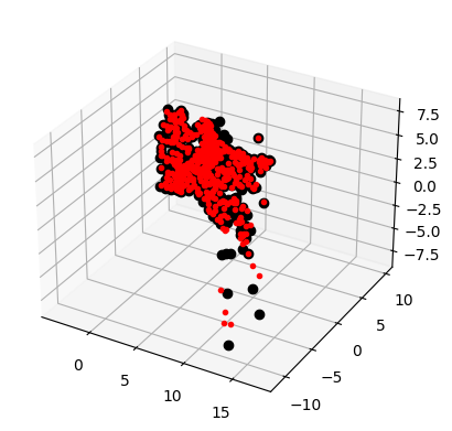 在这里插入图片描述
可以看到，算法估计出的三维图像点和实际图像点很接近。

由三维点计算照相机矩阵

本质上，这是三角剖分的逆问题，有时我们将其称为照相机反切法，恢复照相机矩阵同样是一个最小二乘问题。
按照 $λixi=PXi\boldsymbol{\lambda}_i\mathbf{x}_i\boldsymbol{=}\boldsymbol{P}\mathbf{X}_i$ 投影到 $xi=[xi,yi,1]\mathbf{x}_i{=}[x_i,y_i,1]$ 可得
$[X1T00−x100⋯0X1T0−y100⋯00X1T−100⋯X2T000−x20⋯0X2T00−y20⋯00X2T0−10⋯⋮⋮⋮⋮⋮⋮⋮][p1Tp2Tp3Tλ1λ2⋮]=0\begin{bmatrix}\mathbf{X}_1^T&0&0&-x_1&0&0&\cdots\\0&\mathbf{X}_1^T&0&-y_1&0&0&\cdots\\0&0&\mathbf{X}_1^T&-1&0&0&\cdots\\\mathbf{X}_2^T&0&0&0&-x_2&0&\cdots\\0&\mathbf{X}_2^T&0&0&-y_2&0&\cdots\\0&0&\mathbf{X}_2^T&0&-1&0&\cdots\\\vdots&\vdots&\vdots&\vdots&\vdots&\vdots&\vdots\end{bmatrix}\begin{bmatrix}\mathbf{p}_1^T\\\mathbf{p}_2^T\\\mathbf{p}_3^T\\\lambda_1\\\lambda_2\\\vdots\end{bmatrix}=0$

def compute_P(x,X): 
    n = x.shape[1]
    if X.shape[1] != n:
        raise ValueError("Number of points don't match.")
   # 创建用于计算 DLT 解的矩阵
    M = zeros((3*n,12+n))
    for i in range(n):
        M[3*i,0:4] = X[:,i]
        M[3*i+1,4:8] = X[:,i]
        M[3*i+2,8:12] = X[:,i]
        M[3*i:3*i+3,i+12] = -x[:,i]
        U,S,V = linalg.svd(M)
    return V[-1,:12].reshape((3,4))

最后一个特征向量的前12个元素是照相机矩阵的元素。

下面的代码会选出第一个视图中的一些可见点，将它们转换维齐次坐标表示，然后估计照相机矩阵:

from numpy import *
import scipy
from matplotlib import pyplot as plt
import cv2


class Camera(object):
    """ Class for representing pin-hole cameras. """
    
    def __init__(self,P):
        """ Initialize P = K[R|t] camera model. """
        self.P = P
        # 标定矩阵
        self.K = None # calibration matrix
        self.R = None # rotation
        self.t = None # translation
        # 照相机中心
        self.c = None # camera center
        
    
    def project(self,X):
        """    Project points in X (4*n array) and normalize coordinates. """
        
        #定义和坐标归一化 
        # (3,n)
        x = dot(self.P,X)
        for i in range(3):
            x[i] /= x[2]    
        return x
    def rotation_matrix(self,a):
        """    Creates a 3D rotation matrix for rotation
        around the axis of the vector a. """
        
        # 旋转矩阵
        R = eye(4)
        R[:3,:3] = scipy.linalg.expm([[0,-a[2],a[1]],[a[2],0,-a[0]],[-a[1],a[0],0]])
        return R
    
    def factor(self):
        """    Factorize the camera matrix into K,R,t as P = K[R|t]. """
        
        # 分解前三列
        K,R = scipy.linalg.rq(self.P[:,:3])
        # 分解后三列
        T = diag(sign(diag(K)))
        if linalg.det(T) < 0:
            T[1,1] *= -1
        self.K = dot(K,T)
        self.R = dot(T,R) # T is its own inverse
        self.t = dot(linalg.inv(self.K),self.P[:,3])
        
        return self.K, self.R, self.t
        
        
def my_calibration(sz):
    """
    Calibration function for the camera (iPhone4) used in this example.
    """
    row, col = sz
    fx = 2555*col/2592
    fy = 2586*row/1936
    K = diag([fx, fy, 1])
    K[0, 2] = 0.5*col
    K[1, 2] = 0.5*row
    return K

# 生成齐次坐标
def make_homog(points):
    """Convert points to homogeneous coordinates."""
    return vstack((points,ones((1,points.shape[1])))) 

def normalize(points):
    """ Normalize a collection of points in 
        homogeneous coordinates so that last row = 1. """

    for row in points:
        row /= points[-1]
    return points


def compute_fundamental(x1,x2):
    """ 使用归一化的八点算法，从对应点（x1，x2 3×n 的数组）中计算基础矩阵
    每行由如下构成：
    [x'*x，x'*y' x', y'*x, y'*y, y', x, y, 1]"""
    n = x1.shape[1]

    if x2.shape[1] != n:
        raise ValueError("Number of points don't match.")
    # 创建方程对应的矩阵
    A = zeros((n,9))
    for i in range(n):
        A[i] = [x1[0,i]*x2[0,i], x1[0,i]*x2[1,i], x1[0,i]*x2[2,i],
    x1[1,i]*x2[0,i], x1[1,i]*x2[1,i], x1[1,i]*x2[2,i],
    x1[2,i]*x2[0,i], x1[2,i]*x2[1,i], x1[2,i]*x2[2,i] ]
    # 计算线性最小二乘解
    U,S,V = linalg.svd(A)
    # V的最后一行有9个元素
    F = V[-1].reshape(3,3)
    # 受限 F
    # 通过将最后一个奇异值置 0，使秩为 2
    U,S,V = linalg.svd(F)
    S[2] = 0
    F = dot(U,dot(diag(S),V))
    return F

def compute_epipole(F):
    """ 从基础矩阵 F 中计算右极点（可以使用 F.T 获得左极点）"""
    # 返回 F 的零空间（Fx=0）
    U,S,V = linalg.svd(F)
    e = V[-1]
    # 归一化
    return e/e[2]

def plot_epipolar_line(im,F,x,epipole=None,show_epipole=True):
    """ 在图像中，绘制外极点和外极线 F×x=0。F 是基础矩阵，x 是另一幅图像中的点 """
    m,n = im.shape[:2]
    line = dot(F,x)
    # 外极线参数和值
    t = linspace(0,n,100)
    lt = array([(line[2]+line[0]*tt)/(-line[1]) for tt in t])
    # 仅仅处理位于图像内部的点和线
    ndx = (lt>=0) & (lt<m)
    plt.plot(t[ndx],lt[ndx],linewidth=2)
    if show_epipole:
        if epipole is None:
            epipole = compute_epipole(F)
    plt.plot(epipole[0]/epipole[2],epipole[1]/epipole[2],'r*')




def triangulate_point(x1,x2,P1,P2):
    """ 使用最小二乘解，绘制点对的三角剖分 """
    M = zeros((6,6))
    M[:3,:4] = P1
    M[3:,:4] = P2
    M[:3,4] = -x1
    M[3:,5] = -x2
    U,S,V = linalg.svd(M)
    X = V[-1,:4]
    return X / X[3]

def triangulate(x1,x2,P1,P2):
    """ x1 和 x2（3×n 的齐次坐标表示）中点的二视图三角剖分 """
    n = x1.shape[1]
    if x2.shape[1] != n:
        raise ValueError("Number of points don't match.")
    X = [ triangulate_point(x1[:,i],x2[:,i],P1,P2) for i in range(n)]
    return array(X).T



from PIL import Image
from numpy import *
from pylab import *
# 载入一些图像
im1 = array(Image.open('images/001.jpg'))
im2 = array(Image.open('images/002.jpg'))
# 载入每个视图的二维点到列表中
points2D = [loadtxt('2D/00'+str(i+1)+'.corners').T for i in range(3)]
# 载入三维点
points3D = loadtxt('3D/p3d').T
# 载入对应
corr = genfromtxt('2D/nview-corners',dtype='int')
# 载入照相机矩阵到 Camera 对象列表中
P = [Camera(loadtxt('2D/00'+str(i+1)+'.P')) for i in range(3)]
# 将三维点转换成齐次坐标表示，并投影
X = vstack( (points3D,ones(points3D.shape[1])) )
x = P[0].project(X)










# 前两个视图中点的索引
ndx = (corr[:,0]>=0) & (corr[:,1]>=0)
# 获取坐标，并用齐次坐标表示
x1 = points2D[0][:,corr[ndx,0]]
x1 = vstack( (x1,ones(x1.shape[1])) )
x2 = points2D[1][:,corr[ndx,1]]
x2 = vstack( (x2,ones(x2.shape[1])) )
Xtrue = points3D[:,ndx]
Xtrue = vstack( (Xtrue,ones(Xtrue.shape[1])) )
# 检查前三个点
Xest = triangulate(x1,x2,P[0].P,P[1].P)
print(Xest[:,:3])
print(Xtrue[:,:3])


def compute_P(x,X): 
    n = x.shape[1]
    if X.shape[1] != n:
        raise ValueError("Number of points don't match.")
   # 创建用于计算 DLT 解的矩阵
    M = zeros((3*n,12+n))
    for i in range(n):
        M[3*i,0:4] = X[:,i]
        M[3*i+1,4:8] = X[:,i]
        M[3*i+2,8:12] = X[:,i]
        M[3*i:3*i+3,i+12] = -x[:,i]
        U,S,V = linalg.svd(M)
    return V[-1,:12].reshape((3,4))


corr = corr[:,0] # 视图 1
ndx3D = where(corr>=0)[0] # 丢失的数值为 -1
ndx2D = corr[ndx3D]
# 选取可见点，并用齐次坐标表示
x = points2D[0][:,ndx2D] # 视图 1
x = vstack( (x,ones(x.shape[1])) )
X = points3D[:,ndx3D]
X = vstack( (X,ones(X.shape[1])) )
# 估计 P
Pest = Camera(compute_P(x,X))
# 比较！
print (Pest.P / Pest.P[2,3]) 
print (P[0].P / P[0].P[2,3])
# 投影
xest = Pest.project(X)
# 绘制图像
plt.figure()
plt.imshow(im1)
plt.plot(x[0],x[1],'bo')
plt.plot(xest[0],xest[1],'r.')
plt.axis('off')
plt.show()

在这里插入图片描述

在这里插入图片描述
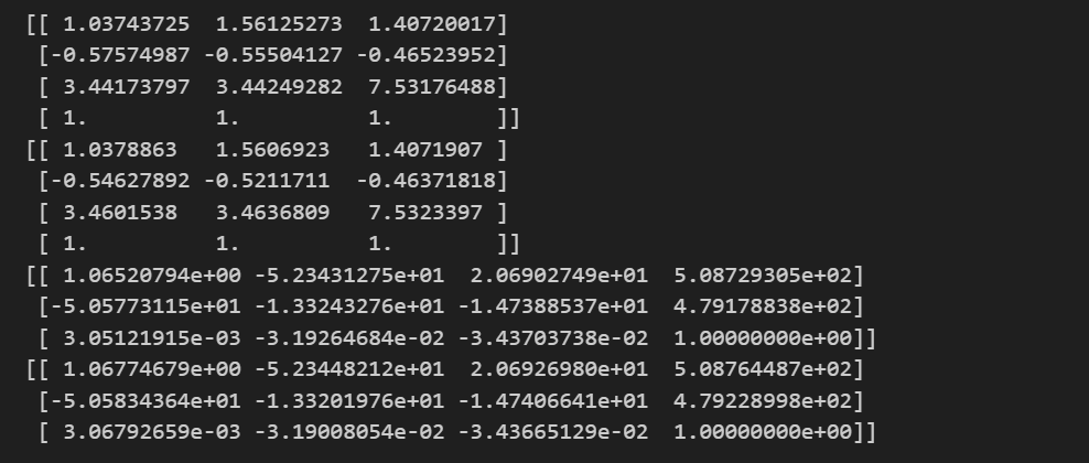
真实点用圆圈表示，照相机矩阵投影点用圆表示，结果基本相同。

多视图重建

假设照相机已经标定，计算重建可以分为下面 4 个步骤：
(1) 检测特征点，然后在两幅图像间匹配；
(2) 由匹配计算基础矩阵；
(3) 由基础矩阵计算照相机矩阵；
(4) 三角剖分这些三维点。

已完成好4个步骤的代码，但当图像间的点对应包含不正确的匹配时，需要一个稳健的方法来计算基础矩阵。

稳健估计基础矩阵

三维重建的四种主要方式：

基于图像。应用广泛，精度比较低。
使用探针或激光读书器逐点获取数据，进行整体三角化，此类方法测量精确，但速度很慢，难以短时间内获得大量数据。
根据三维物体的断层扫面，得到二维图像轮廓，进行相邻轮廓的连接和三角化，得到物体表面形状。
光学三维扫描仪。应用硬件光学三维扫描仪获得物体的点云数据，进行重建获得物体的整体表面信息。

假设照相机已经标定，计算重建可以分为下面 4 个步骤：

检测特征点，然后在两幅图像间匹配；
由匹配计算基础矩阵；
由基础矩阵计算照相机矩阵；
三角剖分这些三维点。

编写代码：

from numpy import *
import scipy
from matplotlib import pyplot as plt
import cv2
# from skimage.measure import ransac


class Camera(object):
    """ Class for representing pin-hole cameras. """
    
    def __init__(self,P):
        """ Initialize P = K[R|t] camera model. """
        self.P = P
        # 标定矩阵
        self.K = None # calibration matrix
        self.R = None # rotation
        self.t = None # translation
        # 照相机中心
        self.c = None # camera center
        
    
    def project(self,X):
        """    Project points in X (4*n array) and normalize coordinates. """
        
        #定义和坐标归一化 
        # (3,n)
        x = dot(self.P,X)
        for i in range(3):
            x[i] /= x[2]    
        return x
    def rotation_matrix(self,a):
        """    Creates a 3D rotation matrix for rotation
        around the axis of the vector a. """
        
        # 旋转矩阵
        R = eye(4)
        R[:3,:3] = scipy.linalg.expm([[0,-a[2],a[1]],[a[2],0,-a[0]],[-a[1],a[0],0]])
        return R
    
    def factor(self):
        """    Factorize the camera matrix into K,R,t as P = K[R|t]. """
        
        # 分解前三列
        K,R = scipy.linalg.rq(self.P[:,:3])
        # 分解后三列
        T = diag(sign(diag(K)))
        if linalg.det(T) < 0:
            T[1,1] *= -1
        self.K = dot(K,T)
        self.R = dot(T,R) # T is its own inverse
        self.t = dot(linalg.inv(self.K),self.P[:,3])
        
        return self.K, self.R, self.t
        
        
def my_calibration(sz):
    """
    Calibration function for the camera (iPhone4) used in this example.
    """
    row, col = sz
    fx = 2555*col/2592
    fy = 2586*row/1936
    K = diag([fx, fy, 1])
    K[0, 2] = 0.5*col
    K[1, 2] = 0.5*row
    return K

# 生成齐次坐标
def make_homog(points):
    """Convert points to homogeneous coordinates."""
    return vstack((points,ones((1,points.shape[1])))) 

def normalize(points):
    """ Normalize a collection of points in 
        homogeneous coordinates so that last row = 1. """

    for row in points:
        row /= points[-1]
    return points


def compute_fundamental(x1,x2):
    """ 使用归一化的八点算法，从对应点（x1，x2 3×n 的数组）中计算基础矩阵
    每行由如下构成：
    [x'*x，x'*y' x', y'*x, y'*y, y', x, y, 1]"""
    n = x1.shape[1]

    if x2.shape[1] != n:
        raise ValueError("Number of points don't match.")
    # 创建方程对应的矩阵
    A = zeros((n,9))
    for i in range(n):
        A[i] = [x1[0,i]*x2[0,i], x1[0,i]*x2[1,i], x1[0,i]*x2[2,i],
    x1[1,i]*x2[0,i], x1[1,i]*x2[1,i], x1[1,i]*x2[2,i],
    x1[2,i]*x2[0,i], x1[2,i]*x2[1,i], x1[2,i]*x2[2,i] ]
    # 计算线性最小二乘解
    U,S,V = linalg.svd(A)
    # V的最后一行有9个元素
    F = V[-1].reshape(3,3)
    # 受限 F
    # 通过将最后一个奇异值置 0，使秩为 2
    U,S,V = linalg.svd(F)
    S[2] = 0
    F = dot(U,dot(diag(S),V))
    return F

def compute_epipole(F):
    """ 从基础矩阵 F 中计算右极点（可以使用 F.T 获得左极点）"""
    # 返回 F 的零空间（Fx=0）
    U,S,V = linalg.svd(F)
    e = V[-1]
    # 归一化
    return e/e[2]

def plot_epipolar_line(im,F,x,epipole=None,show_epipole=True):
    """ 在图像中，绘制外极点和外极线 F×x=0。F 是基础矩阵，x 是另一幅图像中的点 """
    m,n = im.shape[:2]
    line = dot(F,x)
    # 外极线参数和值
    t = linspace(0,n,100)
    lt = array([(line[2]+line[0]*tt)/(-line[1]) for tt in t])
    # 仅仅处理位于图像内部的点和线
    ndx = (lt>=0) & (lt<m)
    plt.plot(t[ndx],lt[ndx],linewidth=2)
    if show_epipole:
        if epipole is None:
            epipole = compute_epipole(F)
    plt.plot(epipole[0]/epipole[2],epipole[1]/epipole[2],'r*')




def triangulate_point(x1,x2,P1,P2):
    """ 使用最小二乘解，绘制点对的三角剖分 """
    M = zeros((6,6))
    M[:3,:4] = P1
    M[3:,:4] = P2
    M[:3,4] = -x1
    M[3:,5] = -x2
    U,S,V = linalg.svd(M)
    X = V[-1,:4]
    return X / X[3]

def triangulate(x1,x2,P1,P2):
    """ x1 和 x2（3×n 的齐次坐标表示）中点的二视图三角剖分 """
    n = x1.shape[1]
    if x2.shape[1] != n:
        raise ValueError("Number of points don't match.")
    X = [ triangulate_point(x1[:,i],x2[:,i],P1,P2) for i in range(n)]
    return array(X).T



from PIL import Image
from numpy import *
from pylab import *
# 载入一些图像
im1 = array(Image.open('images/001.jpg'))
im2 = array(Image.open('images/002.jpg'))
# 载入每个视图的二维点到列表中
points2D = [loadtxt('2D/00'+str(i+1)+'.corners').T for i in range(3)]
# 载入三维点
points3D = loadtxt('3D/p3d').T
# 载入对应
corr = genfromtxt('2D/nview-corners',dtype='int')
# 载入照相机矩阵到 Camera 对象列表中
P = [Camera(loadtxt('2D/00'+str(i+1)+'.P')) for i in range(3)]
# 将三维点转换成齐次坐标表示，并投影
X = vstack( (points3D,ones(points3D.shape[1])) )
x = P[0].project(X)










# 前两个视图中点的索引
ndx = (corr[:,0]>=0) & (corr[:,1]>=0)
# 获取坐标，并用齐次坐标表示
x1 = points2D[0][:,corr[ndx,0]]
x1 = vstack( (x1,ones(x1.shape[1])) )
x2 = points2D[1][:,corr[ndx,1]]
x2 = vstack( (x2,ones(x2.shape[1])) )
Xtrue = points3D[:,ndx]
Xtrue = vstack( (Xtrue,ones(Xtrue.shape[1])) )
# 检查前三个点
Xest = triangulate(x1,x2,P[0].P,P[1].P)
print(Xest[:,:3])
print(Xtrue[:,:3])


def compute_P(x,X): 
    n = x.shape[1]
    if X.shape[1] != n:
        raise ValueError("Number of points don't match.")
   # 创建用于计算 DLT 解的矩阵
    M = zeros((3*n,12+n))
    for i in range(n):
        M[3*i,0:4] = X[:,i]
        M[3*i+1,4:8] = X[:,i]
        M[3*i+2,8:12] = X[:,i]
        M[3*i:3*i+3,i+12] = -x[:,i]
        U,S,V = linalg.svd(M)
    return V[-1,:12].reshape((3,4))

# 从点对中计算 P
class RansacModel(object):
    def __init__(self,debug = False):
        self.debug = debug
        
    def fit(self,data):
        data=data.T
        # 数据分成两个点集,x1分为前三行，x2分为三行之后
        x1 = data[:3,:8]
        x2 = data[3:,:8]
        
        F = compute_fundamental_normalized(x1,x2)
        return F

    def get_error(self,data,F):
        data = data.T
        x1 = data[:3]
        x2 = data[3:]
        # 将 Sampson 距离用作误差度量
        Fx1 = dot(F,x1)
        Fx2 = dot(F,x2)
        denom = Fx1[0]**2 + Fx1[1]**2 + Fx2[0]**2 + Fx2[1]**2
        err = ( diag(dot(x1.T,dot(F,x2))) )**2 / denom
        # 返回每个点的误差
        return err


# 归一化的八点算法
def compute_fundamental_normalized(x1,x2):
    n = x1.shape[1]
    if x2.shape[1] != n:
        raise ValueError("Number of points don't match.")
 # 归一化图像坐标
    x1 = x1 / x1[2]
    mean_1 = mean(x1[:2],axis=1)
    S1 = sqrt(2) / std(x1[:2])
    T1 = array([[S1,0,-S1*mean_1[0]],[0,S1,-S1*mean_1[1]],[0,0,1]])
    x1 = dot(T1,x1)
    x2 = x2 / x2[2]
    mean_2 = mean(x2[:2],axis=1)
    S2 = sqrt(2) / std(x2[:2])
    T2 = array([[S2,0,-S2*mean_2[0]],[0,S2,-S2*mean_2[1]],[0,0,1]])
    x2 = dot(T2,x2)
 # 使用归一化的坐标计算F
    F = compute_fundamental(x1,x2)
 # 反归一化
    F = dot(T1.T,dot(F,T2))
 # F[2,2]是最后一个坐标
    return F/F[2,2]

# 从点对中计算基础矩阵
def F_from_ransac(x1,x2,model,maxiter=5000,match_theshold=1e-6):
    import ransac
    data = vstack((x1,x2))
    # 计算 F 和内点
    F,ransac_data = ransac.ransac(data.T,model,8,maxiter,match_theshold,20,return_all=True)
    return F, ransac_data['inliers']


def compute_P_from_essential(E):
    """ 从本质矩阵计算四个可能的 P 矩阵 """
    # 本质矩阵有两个奇异值，一个为 0，另一个相等
    U,S,V = linalg.svd(E)
    # 两个可能的解
    W = array([[0,-1,0],[1,0,0],[0,0,1]])
    # 两个可能的 P 矩阵
    P2 = [vstack((dot(U,dot(W,V)).T,U[:,2])).T,
    vstack((dot(U,dot(W,V)).T,-U[:,2])).T]
    return P2



# 标定矩阵
K = array([[2394,0,932],[0,2398,628],[0,0,1]])
# 载入图像，并计算特征
im1 = array(Image.open('images/001.jpg').convert('L'))
l1,d1 = cv2.SIFT_create().detectAndCompute(im1,None)
im2 = array(Image.open('images/002.jpg').convert('L'))
l2,d2 = cv2.SIFT_create().detectAndCompute(im2,None)
# 匹配特征，并计算齐次坐标
matches = cv2.BFMatcher().knnMatch(d1,d2,k=2)
ndx = matches[0]
# 去除错误匹配
matches = [m for m,n in matches if m.distance < 0.7*n.distance]
ndx = matches
# 归一化坐标
x1 = make_homog(array([l1[m.queryIdx].pt for m in matches]).T)
ndx2 = [m.trainIdx for m in matches]
x2 = make_homog(array([l2[m.trainIdx].pt for m in matches]).T)

x1n = dot(inv(K),x1)
x2n = dot(inv(K),x2)


model = RansacModel()
E,inliers = F_from_ransac(x1n,x2n,model,maxiter=1000)
P1 = array([[1,0,0,0],[0,1,0,0],[0,0,1,0]])
# 4 个可能的解
P2 = compute_P_from_essential(E)

# 选取点在照相机前的解
ind = 0
maxres = 0
for i in range(4):
    # 三角剖分正确点，并计算每个照相机的深度
    X = triangulate(x1n[:,inliers],x2n[:,inliers],P1,P2[i])
    d1 = dot(P1,X)[2]
    d2 = dot(P2[i],X)[2]

    if sum(d1>0)+sum(d2>0) > maxres:
        maxres = sum(d1>0)+sum(d2>0)
        ind = i
        infront = (d1>0) & (d2>0)
    # 三角剖分正确点，并移除不在所有照相机前面的点
    X = triangulate(x1n[:,inliers],x2n[:,inliers],P1,P2[ind])
    X = X[:,infront]

    # 绘制三维图像
    from mpl_toolkits.mplot3d import axes3d
    fig = figure()
    ax = fig.add_subplot(projection='3d')
    ax.plot(-X[0], X[1], X[2], 'k.')
    axis('off')
    # 绘制 X 的投影 import camera
    # 绘制三维点
    cam1 = Camera(P1)
    cam2 = Camera(P2[ind])
    x1p = cam1.project(X)
    x2p = cam2.project(X)
    # 反 K 归一化
    x1p = dot(K, x1p)
    x2p = dot(K, x2p)
    plt.figure()
    plt.imshow(im1)
    plt.gray()
    plt.plot(x1p[0], x1p[1], 'o')
    plt.plot(x1[0], x1[1], 'r.')
    plt.axis('off')
    plt.figure()
    plt.imshow(im2)
    plt.gray()
    plt.plot(x2p[0], x2p[1], 'o')
    plt.plot(x2[0], x2[1], 'r.')
    plt.axis('off')
    plt.show()

文中提到的链接已经不能用了，新链接参见：https://scipy-cookbook.readthedocs.io/_downloads/d7a553f634786b4ad9b366d80a229e5f/ransac.py

另外，有些代码也已经过时了，需要修改后才能使用。
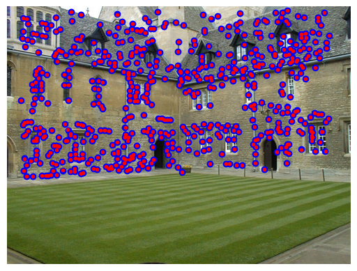
运行结果：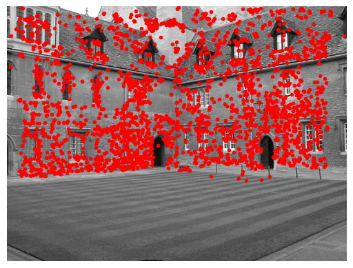
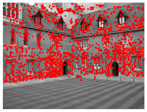
在这里插入图片描述

可以看到，二次投影后的点和原始特征位置不完全匹配，但是已经非常好了。