论文介绍

深度学习在海洋数据推断和亚网格参数化中的应用
Applications of Deep Learning to Ocean Data Inference and Sub-Grid Parameterisation

Fig1，图代码见下图

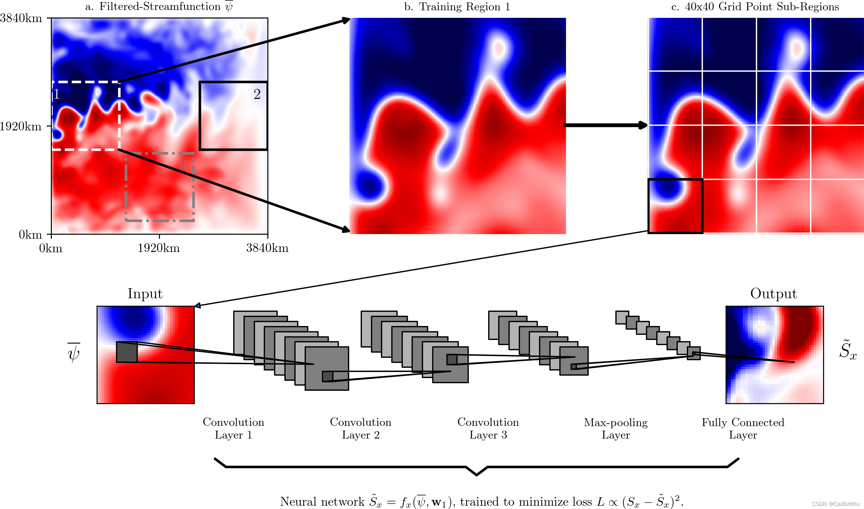
在这张图中，有很多非常有意思的用法，对我们平时做图参考价值非常大。

1 作图，3行3列，大小12:9，也就是4:3的大小

##### Plotting #####
fig, axArr = plt.subplots( 3, 3, figsize=(12,9) )
plt.subplots_adjust( bottom=0.05, top=0.95 )

第一幅图设置，数据绘制，设置，很规整

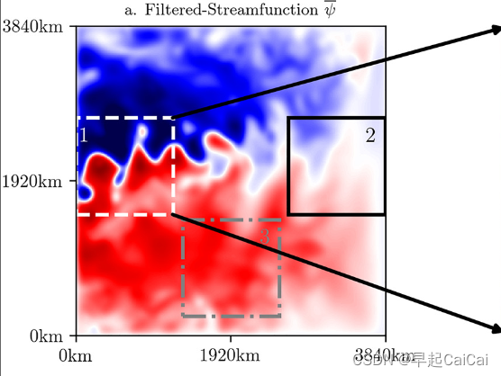
# Psi snapshot with training regions
im0 = axArr[0,0].imshow( psiFilt*1e-5, cmap='seismic', vmin=-cLim, vmax=cLim, origin='lower' )

axArr[0,0].set_title('a. Filtered-Streamfunction $\overline{\psi}$', fontsize=9, fontweight='bold' )
axArr[0,0].set_ylim( (0,512) )
axArr[0,0].set_xlim( (0,512) )
axArr[0,0].set_xticks([0,256,512])
axArr[0,0].set_yticks([0,256,512])
axArr[0,0].set_xticklabels(['0km','1920km','3840km'])
axArr[0,0].set_yticklabels(['0km','1920km','3840km'])

随后绘制小的正方形

# Training region 1
myRect1 = Rectangle( xy=(1,200), width=160, height=160, fill=False, color='white', lw=2, ls='--' )
axArr[0,0].add_patch( myRect1 )
axArr[0,0].text( 7, 320, '1', color='white', fontweight='bold', fontsize=12 )

# Training region 2
myRect2 = Rectangle( xy=(352,200), width=160, height=160, fill=False, color='black', lw=2 )
axArr[0,0].add_patch( myRect2 )
axArr[0,0].text( 480, 320, '2', color='black', fontweight='bold', fontsize=12 )

# Training region 3
myRect3 = Rectangle( xy=(177,31), width=160, height=160, fill=False, color='gray', lw=2, ls='-.' )
axArr[0,0].add_patch( myRect3 )
axArr[0,0].text( 305, 151, '3', color='gray', fontweight='bold', fontsize=12 )

添加区域之间的连接线，这个很少看见别人用到，但这个一般的实用性有很大

# (add lines connecting regions)
con1 = ConnectionPatch( xyA=(1,1), xyB=(160,200),
                        coordsA="data", coordsB="data",
                        axesA=axArr[0,1], axesB=axArr[0,0],
                        color="black", arrowstyle='<|-', linewidth=2 )
con2 = ConnectionPatch( xyA=(1,159), xyB=(160,360),
                        coordsA="data", coordsB="data",
                        axesA=axArr[0,1], axesB=axArr[0,0],
                        color="black", arrowstyle='<|-', linewidth=2 )
con3 = ConnectionPatch( xyA=(1,80), xyB=(159,80),
                        coordsA="data", coordsB="data",
                        axesA=axArr[0,2], axesB=axArr[0,1],
                        color="black", arrowstyle='<|-', linewidth=3 )

简而言之：深度学习使得数据加密
该论文2019年1月4日发表在JAMES期刊上

摘要

摘要

海洋观测受到采样率的限制，而海洋模型则受到有限分辨率和高粘度和扩散系数的限制。因此，来自观测和海洋模型的数据都缺乏快速小尺度的信息。我们需要一些方法来提取信息、外推或放大现有的海洋学数据集，以解释或表示未解决的物理过程。在这里，我们使用机器学习通过预测未解决的湍流过程和海平面下的流场来利用观测和模型数据。作为概念证明，我们对来自高分辨率准地转海洋模式的退化数据训练卷积神经网络。我们证明了卷积神经网络成功地复制了次网格涡旋动量强迫的时空变异性，能够推广到一系列动力学行为，并且能够被迫遵守整体动量守恒。我们的卷积神经网络的训练数据可以被二次采样到原始大小的10–20%，而准确度不会显著降低。Wealso还表明，仅使用海表信息（例如，仅使用卫星测高数据）就可以预测海表下的流场。我们的结果表明，数据驱动的方法可以用于预测亚网格和大规模过程，同时尊重物理原理，即使数据仅限于特定区域或外部强迫。我们的深入研究为在粗分辨率气候模式下成功设计海洋涡旋参数化提供了证据。

简明语言摘要

海洋学观测受到采样率的限制，而海洋模型则受到有限分辨率和高粘度和扩散系数的限制。因此，来自观测的数据和海洋模型都缺乏小尺度和快速尺度的信息。需要一些方法来提取信息，推断或升级现有的海洋学数据集，以解释或表示未解决的物理过程。
我们成功地使用了一种特殊类型的机器学习算法，称为卷积神经网络，以充分利用当前的海洋学数据。

论文中图的说明

"""
Introductory figure to:
- Illustrate the QG model.
- Each of the three training regions.
- The input and output variables of the neural network.
- The convolutional neural network architecture.
"""

import scipy.io as sio
import numpy as np
import matplotlib.pyplot as plt
from matplotlib.patches import Rectangle, ConnectionPatch
from mpl_toolkits.axes_grid1 import make_axes_locatable

plt.rcdefaults()
from matplotlib.lines import Line2D
from matplotlib.collections import PatchCollection

plt.rc('text', usetex=True )
plt.rc('font', family='serif' )

##### Streamfunction and Training Regions ######

t0 = 200

# truth
truth = np.load('../data/Predictions/SxSy_True_str2.npz')
SxTrue, SyTrue = truth['SxT'], truth['SyT']

# predictions
preds = np.load('../data/Predictions/Sx_Pred_R1_str2.npz')
SxPred = preds['SP']

# filtered-streamfunction
psiFilt = np.moveaxis( sio.loadmat('../data/Validation/psiPred_30km.mat')['psiPred_30km'], 2, 0 )
psiFilt = np.squeeze( psiFilt[t0,:,:] )
psiFiltSub = np.squeeze( psiFilt[200:360,0:160] )

##### Plotting #####
fig, axArr = plt.subplots( 3, 3, figsize=(12,9) )
plt.subplots_adjust( bottom=0.05, top=0.95 )

cLim = 1

# Psi snapshot with training regions
im0 = axArr[0,0].imshow( psiFilt*1e-5, cmap='seismic', vmin=-cLim, vmax=cLim, origin='lower' )

axArr[0,0].set_title('a. Filtered-Streamfunction $\overline{\psi}$', fontsize=9, fontweight='bold' )
axArr[0,0].set_ylim( (0,512) )
axArr[0,0].set_xlim( (0,512) )
axArr[0,0].set_xticks([0,256,512])
axArr[0,0].set_yticks([0,256,512])
axArr[0,0].set_xticklabels(['0km','1920km','3840km'])
axArr[0,0].set_yticklabels(['0km','1920km','3840km'])

# Training region 1
myRect1 = Rectangle( xy=(1,200), width=160, height=160, fill=False, color='white', lw=2, ls='--' )
axArr[0,0].add_patch( myRect1 )
axArr[0,0].text( 7, 320, '1', color='white', fontweight='bold', fontsize=12 )

# Training region 2
myRect2 = Rectangle( xy=(352,200), width=160, height=160, fill=False, color='black', lw=2 )
axArr[0,0].add_patch( myRect2 )
axArr[0,0].text( 480, 320, '2', color='black', fontweight='bold', fontsize=12 )

# Training region 3
myRect3 = Rectangle( xy=(177,31), width=160, height=160, fill=False, color='gray', lw=2, ls='-.' )
axArr[0,0].add_patch( myRect3 )
axArr[0,0].text( 305, 151, '3', color='gray', fontweight='bold', fontsize=12 )

#############################################
# Sub-Region Psi
im1 = axArr[0,1].imshow( psiFiltSub*1e-5, cmap='seismic', vmin=-cLim, vmax=cLim, origin='lower' )
axArr[0,1].axis('off')
axArr[0,1].set_title('b. Training Region 1', fontsize=9, fontweight='bold' )

# Sub-Region Psi (with grid)
im2 = axArr[0,2].imshow( psiFiltSub*1e-5, cmap='seismic', vmin=-cLim, vmax=cLim, origin='lower' )
axArr[0,2].set_title('c. 40x40 Grid Point Sub-Regions', fontsize=9, fontweight='bold' )

axArr[0,2].axis('off')
for i in range(4) :
    for j in range(4) :
        Rect = Rectangle(xy=(i * 40, j * 40), width=40, height=40, fill=False, color='white', lw=1 )
        axArr[0, 2].add_patch(Rect)

Rect = Rectangle(xy=(0,0), width=40, height=40, fill=False, color='black', lw=2 )
axArr[0, 2].add_patch(Rect)


# (add lines connecting regions)
con1 = ConnectionPatch( xyA=(1,1), xyB=(160,200),
                        coordsA="data", coordsB="data",
                        axesA=axArr[0,1], axesB=axArr[0,0],
                        color="black", arrowstyle='<|-', linewidth=2 )
con2 = ConnectionPatch( xyA=(1,159), xyB=(160,360),
                        coordsA="data", coordsB="data",
                        axesA=axArr[0,1], axesB=axArr[0,0],
                        color="black", arrowstyle='<|-', linewidth=2 )
con3 = ConnectionPatch( xyA=(1,80), xyB=(159,80),
                        coordsA="data", coordsB="data",
                        axesA=axArr[0,2], axesB=axArr[0,1],
                        color="black", arrowstyle='<|-', linewidth=3 )

axArr[0,1].add_artist( con1 )
axArr[0,1].add_artist( con2 )
axArr[0,2].add_artist( con3 )

##### ARCHITECTURE #####

NumConvMax = 8
NumFcMax = 20
White = 1.
Light = 0.7
Medium = 0.5
Dark = 0.3
Black = 0.


def add_layer(patches, colors, size=24, num=5,
              top_left=[0, 0],
              loc_diff=[3, -3],
              ):
    # add a rectangle
    top_left = np.array(top_left)
    loc_diff = np.array(loc_diff)
    loc_start = top_left - np.array([0, size])
    for ind in range(num):
        patches.append(Rectangle(loc_start + ind * loc_diff, size, size, ec='black', lw=10))
        if ind % 2:
            colors.append(Medium)
        else:
            colors.append(Light)


def add_mapping(patches, colors, start_ratio, patch_size, ind_bgn,
                top_left_list, loc_diff_list, num_show_list, size_list):

    start_loc = top_left_list[ind_bgn] \
        + (num_show_list[ind_bgn] - 1) * np.array(loc_diff_list[ind_bgn]) \
        + np.array([start_ratio[0] * size_list[ind_bgn],
                    -start_ratio[1] * size_list[ind_bgn]])

    end_loc = top_left_list[ind_bgn + 1] \
        + (num_show_list[ind_bgn + 1] - 1) \
        * np.array(loc_diff_list[ind_bgn + 1]) \
        + np.array([(start_ratio[0] + .5 * patch_size / size_list[ind_bgn]) *
                    size_list[ind_bgn + 1],
                    -(start_ratio[1] - .5 * patch_size / size_list[ind_bgn]) *
                    size_list[ind_bgn + 1]])

    patches.append(Rectangle(start_loc, patch_size, patch_size))
    colors.append(Dark)
    patches.append(Line2D([start_loc[0], end_loc[0]],
                          [start_loc[1], end_loc[1]]))
    colors.append(Black)
    patches.append(Line2D([start_loc[0] + patch_size, end_loc[0]],
                          [start_loc[1], end_loc[1]]))
    colors.append(Black)
    patches.append(Line2D([start_loc[0], end_loc[0]],
                          [start_loc[1] + patch_size, end_loc[1]]))
    colors.append(Black)
    patches.append(Line2D([start_loc[0] + patch_size, end_loc[0]],
                          [start_loc[1] + patch_size, end_loc[1]]))
    colors.append(Black)


def labelTop(xy, text, xy_off=[0, 4]):
    axArr[2,0].text(xy[0] + xy_off[0], xy[1] + xy_off[1], text,
             family='sans-serif', size=9)

def labelBot(xy, text, xy_off=[0, 4]):
    axArr[2,0].text(xy[0] + xy_off[0], xy[1] + xy_off[1], text,
             family='sans-serif', size=9, fontweight='bold', ha='center' )

fc_unit_size = 2
layer_width = 50

patches = []
colors = []


pos = axArr[2,0].get_position()
pos = [ pos.x0*1.35, pos.y0*2.5, pos.width*3, pos.height ]
axArr[2,0].set_position( pos )

############################
# conv layers
size_list = [40, 17, 14, 11, 5, 40]
num_list = [1, 16, 8, 8, 8, 1 ]
x_diff_list = [0, layer_width, layer_width, layer_width, layer_width, layer_width]
text_list = ['Input'] + ['Feature maps'] * (len(size_list) - 2) + ['Output']
loc_diff_list = [[4, -2]] * len(size_list)

num_show_list = list(map(min, num_list, [NumConvMax] * len(num_list)))
top_left_list = np.c_[np.cumsum(x_diff_list), np.zeros(len(x_diff_list))]

for ind in range(len(size_list)):

    if (ind > 0) & (ind < 5) :
        add_layer(patches, colors, size=size_list[ind],
                num=num_show_list[ind],
                top_left=top_left_list[ind], loc_diff=loc_diff_list[ind])

    #labelTop(top_left_list[ind], text_list[ind] + '\n{}x{} (x{})'.format(
    #    size_list[ind], size_list[ind], num_list[ind] ) )


############################
# in between layers
start_ratio_list = [ [0.1,0.5], [0.4, 0.8], [0.4, 0.5], [0.4, 0.8], [0.4,0.6] ]
patch_size_list = [8, 4, 4, 2, 1]
ind_bgn_list = range(len(patch_size_list))
text_list = [ 'Convolution\nLayer 1', 'Convolution\nLayer 2', 'Convolution\nLayer 3', 'Max-pooling\nLayer', 'Fully Connected\nLayer' ]
n_param_list = [ 1040, 2056, 1032, 0, 321600 ]

for ind in range(len(patch_size_list)):
    add_mapping(patches, colors, start_ratio_list[ind],
              patch_size_list[ind], ind,
            top_left_list, loc_diff_list, num_show_list, size_list)
    labelBot(top_left_list[ind], text_list[ind], xy_off=[50, -50] )



############################
colors += [0, 1]
collection = PatchCollection(patches, cmap=plt.cm.gray, edgecolors='black' )
collection.set_array(np.array(colors))
axArr[2,0].add_collection(collection)
#plt.tight_layout()
axArr[2,0].axis('equal')
axArr[2,0].axis('off')
axArr[2,1].axis('off')
axArr[2,2].axis('off')

############################

SxTrue = np.squeeze( SxTrue[t0,200:360,0:160] )
SxPred = np.squeeze( SxPred[t0,200:360,0:160] )

# input
axArr[1,0].imshow( psiFiltSub[:40,:40]*1e-5, cmap='seismic', vmin=-cLim, vmax=cLim, origin='lower' )

s = 0.45
dy = 1.3

pos = axArr[1,0].get_position()
pos = [ pos.x0 + 0.05, pos.y0*dy, pos.width*s, pos.height*s ]
axArr[1,0].set_position( pos )
axArr[1,0].text( -10, 20, r'$\overline{\psi}$', fontsize=15, va='center', ha='center' )
axArr[1,0].set_xticks( [] )
axArr[1,0].set_yticks( [] )
axArr[1,0].set_title( r'Input' )

# output
axArr[1,2].imshow( np.squeeze( SxPred[:40,:40] )*1e6, vmin=-3, vmax=3, origin='lower', cmap='seismic' )
axArr[1,2].text( 40+10, 20, r'$\tilde{S}_x$', fontsize=15, va='center', ha='center' )
axArr[1,2].set_xticks( [] )
axArr[1,2].set_yticks( [] )
axArr[1,2].set_title( r'Output' )

axArr[1,1].axis('off')

pos = axArr[1,2].get_position()
pos = [ pos.x0 + 0.08, pos.y0*dy, pos.width*s, pos.height*s ]
axArr[1,2].set_position( pos )

# move CNN to middle
pos2 = axArr[1,0].get_position()
pos0 = axArr[2,0].get_position()
axArr[2,0].set_position( [ pos0.x0, pos2.y0-0.068, pos0.width, pos0.height ] )

# annotate sub-grid to input
pos1 = axArr[0,2].get_position()
pos2 = axArr[1,0].get_position()

axArr[0,2].annotate( '', xy=( 0.268, 0.596 ), xytext=( 0.69, 0.69 ), xycoords='figure fraction',
            arrowprops=dict( arrowstyle='-|>' ) )

# add DIY underbrace
dx, dy = 0.01, 0.01
L = 0.22

x = np.array( [ 0.3-dx, 0.3, 0.3+L, 0.3+L+dx ] )
y = np.array( [ 0.4+dy, 0.4, 0.4, 0.4-dy ] )

x = np.concatenate( (x,x+L+2*dx) )
y = np.concatenate( (y,y[::-1] ) )

plt.plot( x, y, clip_on=False, transform=fig.transFigure, lw=2, color='black', solid_capstyle='round', solid_joinstyle='round' )

# add text
fig = plt.gcf()
plt.text( 0.35, 0.35, r'Neural network $\tilde{S}_x = f_x(\overline{\psi},\mathbf{w}_1)$, trained to minimize loss $L \propto (S_x-\tilde{S}_x)^2$.',
                    transform=fig.transFigure, fontsize=10 )

plt.savefig('intro.png',format='png',dpi=300)

plt.show()

参考

论文链接

Github DeepEddy