
【C4】基于深度学习的心电信号分析
基于深度学习的心电信号分析
★★★ 本文源自AI Studio社区精品项目,【点击此处】查看更多精品内容 >>>
基于深度学习的心电信号分析
一、项目背景
近年来,随着人工智能和算法的发展,以机器学习和深度学习为主的研究技术被 广泛的应用于医疗领域研究中,在推动医疗诊断技术发展的同时,也缓解了城镇医疗资源配比不均衡。随着城镇一体化、人口老龄化的加剧,许多患有慢性心脏疾病的老年人人数增多。因此,在医疗诊断中结合人工智能技术缓解医疗资源紧张和对中老年 人病情有效的预防监测都具有十分重要的研究意义。从机器学习到深度学习的发展, 各种深度经典网络模型在各分支领域均取得不错的成果。相较于机器学习,深度学习能够实现自主学习并挖掘信号的深层次特征,实现对数据的预测和分类。本次研究结合深度学习网络模型,对心电信号进行分析,实现心电信号特征的自动挖掘和识别分类, 并且提高模型在复杂环境下的泛化能力。
二、项目实现
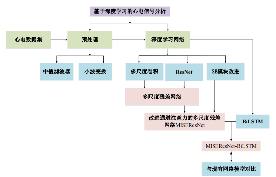
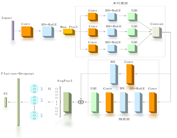
1.研究框架
2.读取数据集
# 加载下载好的库
import sys
sys.path.append('/home/aistudio/external-libraries')
import pywt
import math
import wfdb  # 读取信号工具箱
import pickle
import joblib
import numpy as np
from pywt import wavedec
import scipy.signal as sg
from pathlib import Path  # path方法
from concurrent.futures import ProcessPoolExecutor

PATH = Path("work/data/mit-bih-arrhythmia-database-1.0.0")
sampling_rate = 360

# non-beat labels
invalid_labels = ['|', '~', '!', '+', '[', ']', '"', 'x']
# for correct R-peak location
tol = 0.05
#封装成函数
def sgn(num):
    if(num > 0.0):
        return 1.0
    elif(num == 0.0):
        return 0.0
    else:
        return -1.0

def wavelet_noising(new_df):
    data = new_df
    w = pywt.Wavelet('db5')
    coeffs = pywt.wavedec(data=new_df, wavelet='db5', level=8)
    cA8, cD8,  cD7, cD6, cD5, cD4, cD3, cD2, cD1 = coeffs

    threshold = (np.median(np.abs(cD1)) / 0.6745) * (np.sqrt(2 * np.log(len(cD1))))
    # 将高频信号cD1、cD2置零
    cD1.fill(0)
    # 将其他中低频信号按软阈值公式滤波
    for i in range(1, len(coeffs) - 2):
        coeffs[i] = pywt.threshold(coeffs[i], threshold)
    recoeffs = pywt.waverec(coeffs=coeffs, wavelet='db5')
    return recoeffs

def normalize(data):
    data = np.nan_to_num(data)  # removing NaNs and Infs
    data = data - np.mean(data)
    data = data / np.std(data)
    return data

def worker(record):
    # read ML II signal & r-peaks position and labels
    signal = wfdb.rdrecord((PATH / record).as_posix(), channels=[0]).p_signal[:, 0]

    annotation = wfdb.rdann((PATH / record).as_posix(), extension="atr")
    r_peaks, labels = annotation.sample, np.array(annotation.symbol)
    baseline = sg.medfilt(sg.medfilt(signal, int(0.2 * sampling_rate) - 1), int(0.6 * sampling_rate) - 1)
    filtered_signal = signal - baseline
    filtered_signal = wavelet_noising(filtered_signal)
    # remove non-beat labels
    indices = [i for i, label in enumerate(labels) if label not in invalid_labels]
    # 去除无效心拍后的值
    r_peaks, labels = r_peaks[indices], labels[indices]

    # align r-peaks
    newR = []
    # 对其R峰的位置,R峰对齐的范围[R_tol,R_tol]
    for r_peak in r_peaks:
        r_left = np.maximum(r_peak - int(tol * sampling_rate), 0)
        r_right = np.minimum(r_peak + int(tol * sampling_rate), len(filtered_signal))
        newR.append(r_left + np.argmax(filtered_signal[r_left:r_right]))
    r_peaks = np.array(newR, dtype="int")
    '''归一化心电信号'''
    # remove inter-patient variation
    normalized_signal= normalize(filtered_signal)
    # AAMI categories
    AAMI = {
        "N": 0, "L": 0, "R": 0, "e": 0, "j": 0,  # N
        "A": 1, "a": 1, "S": 1, "J": 1,  # SVEB
        "V": 2, "E": 2,  # VEB
        "F": 3,  # F
        "/": 4, "f": 4, "Q": 4  # Q
    }
    categories = [AAMI[label] for label in labels]

    return {
        "record": record,
        "signal": normalized_signal, "r_peaks": r_peaks, "categories": categories
    }


if __name__ == "__main__":
    # for multi-processing
    cpus = 16 if joblib.cpu_count() > 16 else joblib.cpu_count() - 1

    data = [
        '100', '104', '108', '113', '117', '122', '201', '207', '212', '217', '222', '231',
        '101', '105', '109', '114', '118', '123', '202', '208', '213', '219', '223', '232',
        '102', '106', '111', '115', '119', '124', '203', '209', '214', '220', '228', '233',
        '103', '107', '112', '116', '121', '200', '205', '210', '215', '221', '230', '234'
    ]
    print("train processing...")
    with ProcessPoolExecutor(max_workers=cpus) as executor:
        data = [result for result in executor.map(worker, data)]
    with open((PATH / "mitdb.pkl").as_posix(), "wb") as f:
        #序列化对象,将结果数据流写入到文件对象中,p=4(序列化模式)表示以二进制的形式序列化
        pickle.dump((data ), f, protocol= 4)
    print("ok!")
3.心电信号预处理
心电信号的产生是由于心肌细胞膜内外正负离子运动产生的电位差,由传感器采集仪采集,并通过心电图以波形呈现出来。由于心电信号属于生物电信号,具有低频、低幅值和非线性的特点,在采集过程中极易受到人体内外部噪声干扰。由于噪声来源分布较广,根据产生频率范围及原因,可分为基线漂移、工频干扰、肌电干扰,伪影运动等。值得注意的是,含有噪声的心电信号会应影响模型识别精度,同时也会造成医生的误判。
import os
import pywt
import wfdb
import numpy as np
import scipy.io as io
from scipy import signal
import scipy.signal as sg
import matplotlib.pyplot as plt
from scipy.signal import medfilt
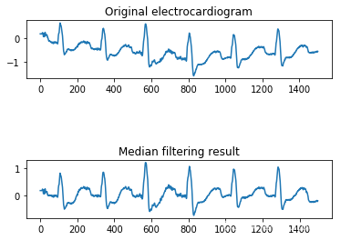
(1)基于中值滤波去除心电信号基线漂移
具体过程为:首先,选取 MIT-BIH 数据库的信号,对其信号点进行排序加窗处理, 窗口先后选用 200ms 和 600ms 来进行低频噪声的去除;其次,对窗口内排好序的中值, 代替原窗口的中心值,这一操作去除掉突出的峰值,信号变得平滑;最后,用原信号减去中值滤波器提取的基线漂移噪声,中值滤波去噪完成。
Initial_intercept_point = 0
Final_intercept_point = 2000
ecg = wfdb.rdrecord('work/data/mit-bih-arrhythmia-database-1.0.0/109', sampfrom=0, sampto=1500, physical=True, channels=[0, ])
ecg = ecg.p_signal.flatten()
index = []
data = []
for i in range(len(ecg)-1):
    X = float(i)
    Y = float(ecg[i])
    index.append(X)
    data.append(Y)
length=len(data)
sampling_rate=360

# filtering uses a 200-ms width median filter and 600-ms width median filter
baseline = sg.medfilt(sg.medfilt(data, int(0.2 * sampling_rate) -1), int(0.6 * sampling_rate)- 1)
filtered_signal = data - baseline
plt.subplot(3, 1,1)
plt.plot(ecg)
plt.title('Original electrocardiogram')
plt.subplot(3, 1, 3)
plt.plot(filtered_signal)  # 显示中值去噪结果
plt.title('Median filtering result')
plt.show()
/opt/conda/envs/python35-paddle120-env/lib/python3.7/site-packages/matplotlib/cbook/__init__.py:2349: DeprecationWarning: Using or importing the ABCs from 'collections' instead of from 'collections.abc' is deprecated, and in 3.8 it will stop working
  if isinstance(obj, collections.Iterator):
/opt/conda/envs/python35-paddle120-env/lib/python3.7/site-packages/matplotlib/cbook/__init__.py:2366: DeprecationWarning: Using or importing the ABCs from 'collections' instead of from 'collections.abc' is deprecated, and in 3.8 it will stop working
  return list(data) if isinstance(data, collections.MappingView) else data
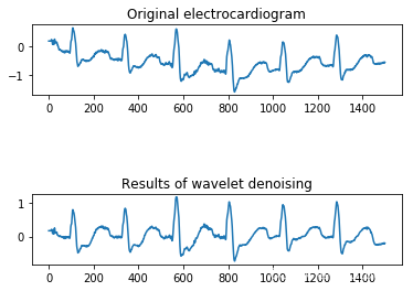
(2)基于离散小波去除心电信号高频噪声
选用 db5 小波对心电信号进行 8 尺度分解,得到包含高频信息和低频信息信号分量,并对 D1 尺度上的高频噪声进行置零操作,将滤除噪声后的心电信号进行重构。
#封装成函数
def sgn(num):
    if(num > 0.0):
        return 1.0
    elif(num == 0.0):
        return 0.0
    else:
        return -1.0

def wavelet_noising(new_df):
    data = new_df
    w = pywt.Wavelet('db5')
    # [ca3, cd3, cd2, cd1] = pywt.wavedec(data, w, level=3)  # 分解波
    coeffs = pywt.wavedec(data=new_df, wavelet='db5', level=7)
    cA7, cD7, cD6, cD5, cD4, cD3, cD2, cD1 = coeffs

    threshold = (np.median(np.abs(cD1)) / 0.6745) * (np.sqrt(2 * np.log(len(cD1))))
    # 将高频信号cD1、cD2置零
    cD1.fill(0)
    #cD2.fill(0)
    # 将其他中低频信号按软阈值公式滤波
    for i in range(1, len(coeffs) - 2):
        coeffs[i] = pywt.threshold(coeffs[i], threshold)
    recoeffs = pywt.waverec(coeffs=coeffs, wavelet='db5')
    return recoeffs
    rdata = rdata

data_denoising = wavelet_noising(filtered_signal)  # 调用小波去噪函数
plt.subplot(3, 1,1)
plt.plot(ecg)
plt.title('Original electrocardiogram')
plt.subplot(3, 1,3)
plt.plot(data_denoising)  # 显示去噪结果
plt.title('Results of wavelet denoising')
plt.show()
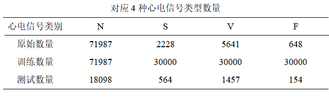
(3)数据集均衡化–SMOTE 算法
依据 AAMI 标准划分的五类心电信号中,Q 类心电信号的准确率仅作参考,因此不考虑对 Q 类进行分类,本次仅对 N、S、V、F 这四种心电信号类型作为模型的输入。但是各类型心电信号样本数之间存在明显的数据不均衡问题,主要是由于心血管患者在人群中占比低, 导致异常心电信号数量少。其中正常 N 类心电信号数量多达 90042,而对 S、V、F 三类异常心电信号样本数较少,严重造成了数据分布极度不均衡现象。数据分布不均衡不利于模型识别并且影响模型最终分类效果,因此为了缓解数据分布不均衡问题带来的影响,使用 SMOTE 算法对少数类样本进行数据增强,使得模型能更充分学习样本特征。SMOTE 算法的基本思想是对异常少数类样本进行分析和拟合,将拟合好后的新样本加入到原始数据集中,实现少数类样本数据扩充,解决了数据不均衡带来的模型识别精度不高的问题。
4.MISEResNet-BiLSTM 网络模型搭建
网络结构
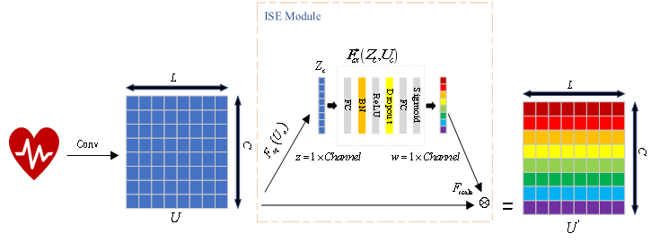
(1)通道注意力机制的改进
传统 SE 模块通过两层全连接层和激活函数一同学习特征通道之间的相关性,本次通过在全连接层中加入了 BN 和 Dropout 来进行部分优化,提出了改进的 ISE(Improved SE)模块, ISE 模块和SE模块不同的地方就是重新加入的 BN 和 Dropout,其中 BN 层用来统一化输入数据分布,且能加快网络运行速度,平滑网络曲线。而 Dropout 具有抑制过拟合作用,并经实验验证参数大小设置为 0.1 效果最佳。通过大量仿真实验验证了 ISE 模块的有效性。
import paddle
import numpy as np
import paddle.nn as nn
import paddle.fluid as fluid
from paddle.nn import initializer

class Shrinkage(nn.Layer):
    def __init__(self,  channel,  reduction=4):
        super(Shrinkage, self).__init__()
        self.gap = nn.AdaptiveAvgPool1D(1)
        self.fc = nn.Sequential(
            nn.Linear(channel, channel//reduction),
            nn.BatchNorm1D(channel//reduction),
            nn.ReLU(),
            nn.Dropout(0.1),
            nn.Linear(channel//reduction, channel),
            nn.Sigmoid(),
        )
    def forward(self, x):
        b, c, _= x.shape
        y1 = self.gap(x).reshape([b, c])
        y = self.fc(y1).reshape([b, c,1])
        return x * y.expand_as(x)
class SpatialAttention(nn.Layer):
    def __init__(self, kernel_size=7):
        super(SpatialAttention, self).__init__()
        assert kernel_size in (3, 7), 'kernel size must be 3 or 7'
        padding = 3 if kernel_size == 7 else 1
        self.conv1 = nn.Conv1D(2, 24, kernel_size, padding=padding, bias_attr=False)
        self.sigmoid = nn.Sigmoid()
    def forward(self, x):
        avg_out = paddle.mean(x, dim=1, keepdim=True)
        max_out, _ = paddle.max(x, dim=1, keepdim=True)
        x = paddle.concat([avg_out, max_out], dim=1)
        x = self.conv1(x)
        return self.sigmoid(x)
class SKConv(nn.Layer):
    def __init__(self, in_channels, out_channels, stride=1, M=2, r=2, L=32):
        super(SKConv, self).__init__()
        d = max(in_channels // r, L)  # 计算向量Z 的长度d
        self.M = M
        self.out_channels = out_channels
        self.conv = nn.ModuleList()  # 根据分支数量 添加 不同核的卷积操作
        for i in range(M):
            # 为提高效率,原论文中 扩张卷积5x5为 (3X3,dilation=2)来代替。 且论文中建议组卷积G=32
            self.conv.append(nn.Sequential(
                nn.Conv1D(in_channels, out_channels, 3, stride, padding=1 + i, dilation=1 + i, groups=32,bias_attr=False),
                nn.BatchNorm1D(out_channels),
                nn.ReLU(inplace=True)))
        self.global_pool = nn.AdaptiveAvgPool1D(1)  # 自适应pool到指定维度    这里指定为1,实现 GAP
        self.fc1 = nn.Sequential(nn.Conv1D(out_channels, d, 1, bias_attr=False),
                                 nn.BatchNorm1D(d),
                                 nn.ReLU())  # 降维
        self.fc2 = nn.Conv1D(d, out_channels * M, 1, 1, bias_attr==False)  # 升维
        self.softmax = nn.Softmax(dim=1)  # 指定dim=1  使得两个全连接层对应位置进行softmax,保证 对应位置a+b+..=1

    def forward(self, input):
        batch_size = input.size(0)
        output = []
        # the part of split
        for i, conv in enumerate(self.conv):
            output.append(conv(input))
        # the part of fusion
        U = reduce(lambda x, y: x + y, output)  # 逐元素相加生成 混合特征U
        s = self.global_pool(U)
        z = self.fc1(s)  # S->Z降维
        a_b = self.fc2(z)  # Z->a,b 升维  论文使用conv 1x1表示全连接。结果中前一半通道值为a,后一半为b
        a_b = a_b.reshape(batch_size, self.M, -1)  # 调整形状,变为 两个全连接层的值
        a_b = self.softmax(a_b)  # 使得两个全连接层对应位置进行softmax
        a_b = list(a_b.chunk(self.M, dim=1))  # split to a and b   chunk为pytorch方法,将tensor按照指定维度切分成 几个tensor块
        a_b = list(map(lambda x: x.reshape(batch_size, self.out_channels, 1), a_b))  # 将所有分块  调整形状,即扩展两维
        V = list(map(lambda x, y: x * y, output, a_b))  # 权重与对应  不同卷积核输出的U 逐元素相乘
        V = reduce(lambda x, y: x + y, V)  # 两个加权后的特征 逐元素相加
        return V
ISE 模块结构图
( 2)ResNet 网络
ResNet 是何凯明等人在 2015 年提出的,并在 Imagenet 的分类任务竞赛中获得第 一名。由于它的可移植性较强,在边缘检测,图像分割,语音识别等领域里得到广泛 的应用。该网络是由多个残差模块构成,通过堆叠多个残差模块使得网络在扩增到 100 层、1000 层时性能得到提升的同时不损失精确度。
class ResBlk(nn.Layer):
    expansion=1
    def __init__(self,in_channel,out_channel,stride=1,downsample=None):
        '''downsample对应虚线残差结构'''
        super(ResBlk,self).__init__()
        self.downsample=downsample
        self.conv1=nn.Conv1D( in_channel, out_channel,kernel_size=3,stride=stride,padding=1 )
        self.bn1=nn.BatchNorm1D(out_channel)
        self.relu=nn.ReLU()
        self.conv2=nn.Conv1D(in_channels=out_channel,out_channels=out_channel,
                             kernel_size=3,stride=1,padding=1,bias_attr=False)
        self.bn2=nn.BatchNorm1D(out_channel)
        self.se=Shrinkage(out_channel)
        self.sa=SpatialAttention()
        if self.downsample:
           self.downsample = nn.Sequential(

                       nn.Conv1D(in_channels=in_channel, out_channels=out_channel , kernel_size=1, stride=stride, bias_attr=False),
                       nn.BatchNorm1D(out_channel),
            )
    def forward(self,x):
        identity=x
        if self.downsample is not None:#虚线部分的残差结构,需要下采样 stride=2的pooling
            identity=self.downsample(x)#捷径分支,short cut
        #残差块中的第一个卷积层
        out=self.conv1(x)
        out=self.relu(self.bn1(out))
        #残差块中的第二个卷积层
        out=self.conv2(out)
        out=self.bn2(out)
        out+=identity
        out=self.relu(out)
        out=self.se(out)+identity
        return out
'''resnet50/101/152的残差结构,用的是1*1+3*3+1*1的卷积'''
class Bottleneck(nn.Layer):
    expansion=4
    def __init___(self,in_channel,out_channel,stride=1,downsample=None):
        super(Bottleneck,self).__init__()
        '''第一层卷积层,使用1*1的卷积核,stride=1,未使用padding'''
        self.conv1=nn.Conv1D(in_channels=in_channel,out_channels=out_channel,
                             kernel_size=1,stride=1,bias_attr=False)
        self.bn1=nn.BatchNorm1D(out_channel)
        '''第二层卷积层,使用3*3的卷积核,stride=2,padding=1'''
        self.drop1=nn.Dropout(0)
        self.conv2=nn.Conv1D(in_channels=out_channel,out_channels=out_channel,
                             kernel_size=3,stride=stride,padding=1,bias_attr=False)
        self.bn2=nn.BatchNorm1D(out_channel)
        '''第三层卷积层,使用1*1的卷积核,stride=1'''
        self.drop2=nn.Dropout(0)
        self.conv3=nn.Conv1D(in_channels=out_channel,out_channels=out_channel*self.expansion,
                             kernel_size=1,stride=1,bias_attr=False)
        self.bn3=nn.BatchNorm1D(out_channel*self.expansion)
        self.relu=nn.LeakyReLU()
        self.drop4=nn.Dropout(0)
        self.downsample=downsample
    def forward(self,x):
        identity=x
        if self.downsample is not None:
            identity=self.downsample(x)#捷径分支 short cut
        out=self.conv1(x)
        out=self.bn1(out)
        out=self.relu(out)
        out=self.drop1(out)
        out=self.conv2(out)
        out=self.bn2(out)
        out=self.relu(out)
        out=self.drop2(out)
        out=self.conv3(out)
        out=self.bn3(out)
        out+=identity
        out=self.relu(out)
        return out
(3)多尺度残差网络模型设计
借鉴 inception网络模型,设计了卷积核大小为 3x1,5x1,7x1 的三个分支,用于获取心电信号的多尺度特征。考虑到心电信号属于一维信号,因此设计了一维多尺度残差网络模型用于心电信号的识 别分类,该网络模型主要包括输入层、起始卷积层、多尺度特征提取层、残差网络层, 全连接层。
(4)双向长短时记忆网络
针对心电信号属于时间 序列特征,结合了双向长短时记忆网络模型一起用于心电信号的分类识别
class ResNet(nn.Layer):
    def __init__(self,block,block_num,num_classes=4,include_top=True,num_group=32):
        super(ResNet,self).__init__()
        self.include_top=include_top
        self.in_channel=24
        #-----------输入网络之前--------------------------
        self.conv1=nn.Conv1D(1,out_channels=self.in_channel,kernel_size=7,stride=2,padding=3,bias_attr=False)
        self.bn1=nn.BatchNorm1D(self.in_channel)
        self.relu=nn.ReLU()
        "------------------多尺度卷积模块---------------------"
        self.cnn1 = nn.Sequential(nn.Conv1D(self.in_channel,8, kernel_size=3, stride=1, padding=1),
                                  nn.BatchNorm1D(8),
                                  nn.ReLU()
                                  )
        self.cnn2 = nn.Sequential(nn.Conv1D(self.in_channel, out_channels=8, kernel_size=5, stride=1, padding=2),
                                  nn.BatchNorm1D(8),
                                  nn.ReLU()
                                  )
        self.cnn3 = nn.Sequential(nn.Conv1D(self.in_channel, out_channels=8, kernel_size=7, stride=1, padding=3),
                                  nn.BatchNorm1D(8),
                                  nn.ReLU()
        )
        "-------------LSTM(双向长短时记忆网络)循环卷积网络--------------"
        self.rnn_layer = nn.LSTM(  # 1:bilstm,hidden_size=64,效果仍旧是s,f类的precision不高
            # lstm:hidden_size=32
            input_size=9,
            hidden_size=32,
            num_layers=1,
            direction='bidirectional',
            time_major=False,
            dropout=0,
        )
        self.se1=Shrinkage(8)
        self.sa1=SpatialAttention()
        self.maxpool=nn.MaxPool1D(kernel_size=3,stride=2,padding=1)
        self.layer1=self._make_layer(block,64, block_num[0])#第一个模块结构
        self.layer2=self._make_layer(block,64,block_num[1] ,stride=2)#第二个模块结构
        self.layer3=self._make_layer(block,64,block_num[2], stride=2)#第三个模块结构
        self.layer4=self._make_layer(block,64,block_num[3],stride=2)#第四个模块结构
        self.softmax = nn.Softmax(-1)
        self.dropout = nn.Dropout(0.3)
        if self.include_top:
            self.avgpool=nn.AvgPool1D(1,stride=1)
            self.fc=nn.Linear(64*64*block.expansion,num_classes)
        for m in self.sublayers():
            if isinstance(m, paddle.nn.Conv1D):
                paddle.nn.initializer.KaimingNormal()
    def _make_layer(self,block,channel,block_num, stride=1):
        downsample=None
        if stride!=1 or self.in_channel !=channel*block.expansion:
            downsample=nn.Sequential(
                nn.Conv1D(self.in_channel,channel*block.expansion,
                          kernel_size=1,stride=stride,bias_attr=False),
                nn.BatchNorm1D(channel*block.expansion))#此处用于处理输入特征图
        layers=[]
        layers.append(block(self.in_channel,channel,downsample=downsample,stride=stride ))
        self.in_channel=channel*block.expansion
        for _ in range(1,block_num):
            layers.append(block(self.in_channel,channel ))
        return nn .Sequential(*layers)
    def forward(self,x):
        x1=self.relu(self.bn1(self.conv1(x)))
        x=self.maxpool(x1)
        output1 = self.cnn1(x)
        output1=self.se1(output1)
        output2 = self.cnn2(x)
        output2=self.se1(output2)
        output3 = self.cnn3(x)
        output3=self.se1(output3)
        output3=self.dropout(output3)
        x = paddle.concat([output1, output2, output3], axis=1)
        x=self.layer1(x)
        x = self.dropout(x)
        x=self.layer2(x)
        x = self.dropout(x)
        x=self.layer3(x)
        x = self.dropout(x)
        x=self.layer4(x)
        x = self.dropout(x)
        if self.include_top:
            x=self.avgpool(x)
            x,_=self.rnn_layer(x)
            x=paddle.flatten(x,1)
            x = self.dropout(x)
            x=self.fc(x)
        return x

    def resnet18(num_classes=4,include_top=True):
        return ResNet(ResBlk,[2,2,2,2],num_classes=num_classes,include_top=include_top)
def count_parameters(model):
    return sum(p.numel() for p in model.parameters() if p.requires_grad)

model= ResNet.resnet18()
paddle.summary(model,(-1,1,280))
5.模型训练
import os
import sys
import time
import joblib
import random
import paddle
import numpy as np
import PIL.Image as Image
from functools import partial
import matplotlib.pyplot as plt
import paddle.optimizer as optim
from imblearn.over_sampling import SMOTE
from paddle.optimizer.lr import StepDecay
from paddle.io import DataLoader,TensorDataset
from sklearn.model_selection import train_test_split
os.environ["TF_CPP_MIN_LOG_LEVEL"] = '2'

# 设置随机数
seed = 0
paddle.seed(seed)
np.random.seed(seed)
random.seed(seed)
'''连续小波变换需要的参数'''
def worker(data):
    # heartbeat segmentation interval
    before, after =120 , 160
    #print(coeffs.shape)# (100,650000)
    r_peaks, categories = data["r_peaks"], data["categories"]
    record=data[ "signal"]#(650000,)

    x1,y= [], []
    for i in range(len(r_peaks)):
        if i == 0 or i == len(r_peaks) - 1:
            continue
        if categories[i] == 4:  # remove AAMI Q class
            continue
        x1.append(record[ r_peaks[i] - before: r_peaks[i] + after ]) #(1861,200)
        y.append(categories[i])#(1861,),(1761,),(2025,),(2530,)
    return x1, y
tic = time.time()

#中值滤波
def load_data(filename="work/data/mit-bih-arrhythmia-database-1.0.0/mitdb.pkl"):
    import pickle
    from sklearn.preprocessing import RobustScaler
    with open(filename, "rb") as f:
        train_data = pickle.load(f)

    cpus = 16 if joblib.cpu_count() > 16 else joblib.cpu_count() - 1  # for multi-process

    # for training
    x1_train,  y_train = [], []
    for x1,  y in map(partial(worker), train_data):

        x1_train.append(x1)#(1,1861,100,100)

        y_train.append(y)#(1,1861)

    x1_train = np.expand_dims(np.concatenate(x1_train, axis=0), axis=1).astype(np.float32)
    y_train = np.concatenate(y_train, axis=0).astype(np.int64)

    return x1_train,y_train
X,Y=load_data(filename="work/data/mit-bih-arrhythmia-database-1.0.0/mitdb.pkl")
x_train, x_test, y_train, y_test = train_test_split(X, Y, test_size=0.2, random_state=42)

'''Over_sampling'''
x_train = np.reshape(x_train, [x_train.shape[0] * x_train.shape[1], -1])
# print('x_train',x_train.shape)#(80504,200)
classes = np.unique(y_train)
print('class',classes)
nums = []
for cl in classes:
    ind = np.where(classes == cl)[0][0]
    nums.append(len(np.where(y_train.flatten() == ind)[0]))  # [71987, 2228, 5641, 648]
print(nums)
n_oversampling =30000
ratio = {0: nums[0], 1:n_oversampling, 2:20000, 3:n_oversampling}

# 数据扩增
sm = SMOTE(random_state=12, sampling_strategy=ratio)
x_train, y_train = sm.fit_resample(x_train, y_train)
print('smote:',x_train.shape)#(101987,200)
x_train = np.reshape(x_train, [-1, x_test.shape[1], x_test.shape[2]])  # (101987,1,200)
# print(X_train.shape)
print('Classes in the training set: ', classes)
for cl in classes:
    ind = np.where(classes == cl)[0][0]
    print(cl, len(np.where(y_train.flatten() == ind)[0]))
X_train = paddle.to_tensor(x_train)
print('x_train.shape',X_train.shape)

# 设置训练集和测试集
X_test = paddle.to_tensor(x_test)
Y_train = paddle.to_tensor(y_train)
Y_test = paddle.to_tensor(y_test)
train_db = TensorDataset([X_train, Y_train])
test_db = TensorDataset([X_test, Y_test])
toc = time.time()
print('Time for data processing--- '+str(toc-tic)+' seconds---')

test_flag = False #测试标志,True时加载保存好的模型进行测试

save_dir = "/home/aistudio/work/weight" # 存储权重的路径
#在监控指标没有提升的情况下,epochs 等待轮数。等待大于该值监控指标始终没有提升,则提前停止训练。
patience = 5
batchsize =256
lr =0.00001
epochs =100
#批次大小
batch_size = 64
#动量法系数
momentum = 0
#权重衰减
weight_decay = 5e-4

'''利用 Dataloader加载数据集'''
train_load = DataLoader(train_db, batch_size=batchsize, shuffle=True )
source_batch, target_batch = iter(train_load).next()
print('source_batch:', source_batch.shape, 'target_batch:', target_batch.shape)
test_load = DataLoader(test_db, batch_size=batchsize, shuffle=True )
dataloaders = {
    "train": train_load,
    "validation": test_load
}
model1=paddle.Model(model)
# 设定可视化工具VisualDL的日志数据保存路径
visualdl = paddle.callbacks.VisualDL(log_dir='visualdl_log')
# 只保存验证集准确率最高的模型,即最优模型
class SaveBestModel(paddle.callbacks.Callback):
    def __init__(self, target=0.5, path='./home/aistudio/work/best-model/best_model', verbose=0):
        self.target = target
        self.epoch = None
        self.path = path

    def on_epoch_end(self, epoch, logs=None):
        self.epoch = epoch

    def on_eval_end(self, logs=None):
        if logs.get('acc') > self.target:
            self.target = logs.get('acc')
            self.model.save(self.path)
            print('best acc is {} at epoch {}'.format(self.target, self.epoch))
callback_savebestmodel = SaveBestModel(target=0.5, path='./home/aistudio/work/best-model/best_model')
# 训练数据给我们提供了后续分析训练过程的历史记录,因此保存训练过程中的数据非常重要
import csv
class SaveTrainingData(paddle.callbacks.Callback):
    def __init__(self, data_filepath=''):
        self.data_filepath = data_filepath

    def on_train_begin(self, logs=None):
        file = open(self.data_filepath, 'w', newline='')
        writer = csv.writer(file)
        writer.writerow(['time', 'training_accuracy'])
        writer.writerow([0.0, 0.0])
        file.close()

        self.train_start_time = time.time()

    def on_epoch_end(self, epoch, logs={}):
        total_time = time.time() - self.train_start_time
        file = open(self.data_filepath, 'a')
        writer = csv.writer(file)
        writer.writerow([round(total_time,1), round(logs['acc'], 4)])
        file.close()

if not os.path.exists('training_data'):
    os.mkdir('training_data')
callback_savetrainingdata = SaveTrainingData(data_filepath="training_data/result.csv")

# 设置优化器
optim = paddle.optimizer.Adam(learning_rate=lr, parameters=model.parameters())
 #早期停止

# 准备模型
model1.prepare(optim,loss =paddle.nn.CrossEntropyLoss(),metrics=paddle.metric.Accuracy())
# 开始训练
model1.fit(train_load,test_load,epochs=epochs,batch_size=batch_size,save_dir=save_dir, verbose=1, callbacks=[visualdl,callback_savebestmodel,callback_savetrainingdata])
6.模型评估
#模型验证及测试
best_model_path = "home/aistudio/work/best-model/best_model.pdparams"
NET_MNIST =ResNet.resnet18()
model = paddle.Model(NET_MNIST)
model.load(best_model_path)
model.prepare(optim,paddle.nn.CrossEntropyLoss(),paddle.metric.Accuracy())
#用最好的模型在测试集上验证
results = model.evaluate(test_load, batch_size=batch_size, verbose=1)
print(results)
Eval begin...
step 80/80 [==============================] - loss: 0.1042 - acc: 0.9849 - 34ms/step
Eval samples: 20273
{'loss': [0.10420333], 'acc': 0.9849060326542692}
三.实验结果分析
1. 混淆矩阵检验
本实验用混淆矩阵形式给出了 MISEResNet-BiLSTM 网络的心电信号分类结果。MISEResNet-BiLSTM 网络模型通过反向传播逐层计算权重梯度,并使用梯度下降监督网络学习过程,通过 Softmax 分类器完成心电信号分类,得到的实验结果如下运行结果所示,其中 0、1、2、3 分别对应 N、S、V、F 类四类心电信号。
import time
import paddle
import joblib
import numpy as np
import paddle.fluid as fluid
from functools import partial
from prettytable import PrettyTable
from matplotlib import pyplot  as plt
from paddle.io import DataLoader,TensorDataset
from sklearn.model_selection import train_test_split

class ConfusionMatrix(object):
    def __init__(self, num_classes: int, labels: list):
        self.matrix = np.zeros((num_classes, num_classes))
        self.num_classes = num_classes
        self.labels = labels

    def update(self, preds, labels):
        for p, t in zip(preds, labels):
            self.matrix[p, t] += 1

    def summary(self):
        sum_TP = 0
        for i in range(self.num_classes):
            sum_TP += self.matrix[i, i]
        acc = sum_TP / np.sum(self.matrix)
        print("the model accuracy is ", acc)

        # precision, recall, specificity
        table = PrettyTable()
        table.field_names = ["", "Recall", "Specificity", "Precision"]
        for i in range(self.num_classes):
            TP = self.matrix[i, i]
            FP = np.sum(self.matrix[i, :]) - TP
            FN = np.sum(self.matrix[:, i]) - TP
            TN = np.sum(self.matrix[:, :]) - TP - FP - FN
            Recall = round(TP / (TP + FN), 4) if TP + FN != 0 else 0.
            Specificity = round(TN / (TN + FP), 4) if TN + FP != 0 else 0.
            Precision = round(TP / (TP + FP), 4) if TP + FP != 0 else 0.
            table.add_row([self.labels[i], Recall, Specificity, Precision])
        print(table)

    def plot(self):
        matrix = self.matrix
        print(matrix)
        plt.imshow(matrix, cmap=plt.cm.Blues)

        # 设置x轴坐标label
        plt.xticks(range(self.num_classes), self.labels, rotation=45)
        # 设置y轴坐标label
        plt.yticks(range(self.num_classes), self.labels)
        # 显示colorbar
        plt.colorbar()
        plt.xlabel('predict label')
        plt.ylabel('true label')
        plt.title('Confusion matrix')

        # 在图中标注数量/概率信息
        thresh = matrix.max() / 2
        for x in range(self.num_classes):
            for y in range(self.num_classes):
                # 注意这里的matrix[y, x]不是matrix[x, y]
                info = int(matrix[x, y])
                plt.text(x, y, info,
                         verticalalignment='center',
                         horizontalalignment='center',
                         color="white" if info > thresh else "black")
        plt.tight_layout()
        plt.show()

if __name__ == '__main__':
    # --------------------- 数据载入和整理 -------------------------------
    def worker(data):
        before, after = 120, 160
        r_peaks, categories = data["r_peaks"], data["categories"]
        record = data["signal"]  # (650000,)
        x1, y = [], []
        for i in range(len(r_peaks)):
            if i == 0 or i == len(r_peaks) - 1:
                continue

            if categories[i] == 4:  # remove AAMI Q class
                continue

            x1.append(record[r_peaks[i] - before: r_peaks[i] + after])  # (1861,200)
            y.append(categories[i])  # (1861,),(1761,),(2025,),(2530,)

        return x1, y

    tic = time.time()

    def load_data(filename="/home/aistudio/work/data/mit-bih-arrhythmia-database-1.0.0/mitdb.pkl"):
        import pickle
        from sklearn.preprocessing import RobustScaler

        with open(filename, "rb") as f:
            train_data = pickle.load(f)

        cpus = 16 if joblib.cpu_count() > 16 else joblib.cpu_count() - 1  # for multi-process

        # for training
        x1_train,  y_train = [], []
        for x1,  y in map(partial(worker), train_data):

            x1_train.append(x1)#(1,1861,100,100)
            y_train.append(y)#(1,1861)

        x1_train = np.expand_dims(np.concatenate(x1_train, axis=0), axis=1).astype(np.float32)
        y_train = np.concatenate(y_train, axis=0).astype(np.int64)

        return x1_train,y_train
    X, Y = load_data(filename="/home/aistudio/work/data/mit-bih-arrhythmia-database-1.0.0/mitdb.pkl")
    X_train, X_test, y_train, y_test = train_test_split(X, Y, test_size=0.2, random_state=42)
    X_train = paddle.to_tensor(X_train)
    X_test = paddle.to_tensor(X_test)
    Y_train = paddle.to_tensor(y_train)
    Y_test = paddle.to_tensor(y_test)
    train_db = TensorDataset([X_train, Y_train])
    test_db = TensorDataset([X_test, Y_test])
    batch_size=64
    test_load = DataLoader(test_db, batch_size=batch_size, shuffle=True )
    toc = time.time()
    print('Time for data processing--- ' + str(toc - tic) + ' seconds---')
    # ============================ step 2/5 模型 ============================

    model_path = 'home/aistudio/work/best-model/best_model.pdparams'
    model= ResNet.resnet18()
    para_state_dict = paddle.load(model_path)
    model.set_dict(para_state_dict)

    target_class= np.unique(Y)#0:N,1:S,2:V,3:F,4:Q
    labels = list(target_class)
    confusion = ConfusionMatrix(num_classes=4, labels=labels)
    model.eval()
    with paddle.no_grad():
        for i, (x, label) in enumerate(test_load):
            x, label = x, label
            output = model(x)
            pred = output.argmax(1)
            confusion.update(pred.numpy(), label.numpy())
    confusion.plot()
 tic) + ' seconds---')
    # ============================ step 2/5 模型 ============================

    model_path = 'home/aistudio/work/best-model/best_model.pdparams'
    model= ResNet.resnet18()
    para_state_dict = paddle.load(model_path)
    model.set_dict(para_state_dict)

    target_class= np.unique(Y)#0:N,1:S,2:V,3:F,4:Q
    labels = list(target_class)
    confusion = ConfusionMatrix(num_classes=4, labels=labels)
    model.eval()
    with paddle.no_grad():
        for i, (x, label) in enumerate(test_load):
            x, label = x, label
            output = model(x)
            pred = output.argmax(1)
            confusion.update(pred.numpy(), label.numpy())
    confusion.plot()
    confusion.summary()
Time for data processing--- 1.0500760078430176 seconds---
[[1.7928e+04 3.6000e+01 3.3000e+01 1.4000e+01]
 [8.4000e+01 5.2200e+02 6.0000e+00 0.0000e+00]
 [3.4000e+01 5.0000e+00 1.3820e+03 5.0000e+00]
 [5.2000e+01 1.0000e+00 3.6000e+01 1.3500e+02]]


/opt/conda/envs/python35-paddle120-env/lib/python3.7/site-packages/matplotlib/cbook/__init__.py:2349: DeprecationWarning: Using or importing the ABCs from 'collections' instead of from 'collections.abc' is deprecated, and in 3.8 it will stop working
  if isinstance(obj, collections.Iterator):
/opt/conda/envs/python35-paddle120-env/lib/python3.7/site-packages/matplotlib/cbook/__init__.py:2366: DeprecationWarning: Using or importing the ABCs from 'collections' instead of from 'collections.abc' is deprecated, and in 3.8 it will stop working
  return list(data) if isinstance(data, collections.MappingView) else data
/opt/conda/envs/python35-paddle120-env/lib/python3.7/site-packages/matplotlib/image.py:425: DeprecationWarning: np.asscalar(a) is deprecated since NumPy v1.16, use a.item() instead
  a_min = np.asscalar(a_min.astype(scaled_dtype))
/opt/conda/envs/python35-paddle120-env/lib/python3.7/site-packages/matplotlib/image.py:426: DeprecationWarning: np.asscalar(a) is deprecated since NumPy v1.16, use a.item() instead
  a_max = np.asscalar(a_max.astype(scaled_dtype))
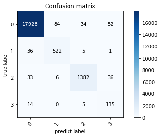
the model accuracy is  0.9849060326542692
+---+--------+-------------+-----------+
|   | Recall | Specificity | Precision |
+---+--------+-------------+-----------+
| 0 | 0.9906 |    0.9618   |   0.9954  |
| 1 | 0.9255 |    0.9954   |   0.8529  |
| 2 | 0.9485 |    0.9977   |   0.9691  |
| 3 | 0.8766 |    0.9956   |   0.6027  |
+---+--------+-------------+-----------+
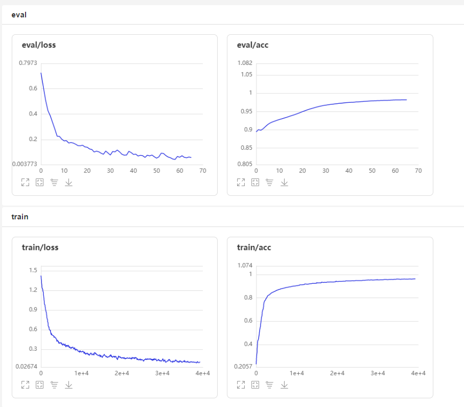
2. 可视化展示
3.与其他文献对比
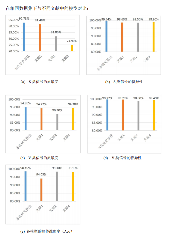
对比文献:
[1]Acharya U R, Oh S L, Hagiwara Y, et al. A deep convolutional neural network model to classify heartbeats[J]. Computers in Biology and Medicine, 2017, 89: 389-396.
[2]Ince, S.Kiranyaz and M. Gabbouj, A generic and robust system for automated patient-specic classication of ECG signals, IEEE Trans. Biomed. Eng. 56 (2009) 1415 –1426.
[3]W. Jiang and S. G. Kong, Block-based neural networks for personalized ECG signalclassication, IEEE Trans. Neural. Netw. 18 (2007) 1750–1761.
四.总结
虽然在上述研究中取得了阶段性的成果,但我们所作仍有许多局限。在未来,为了我们的项目能够切实应用到医疗系统,为患者提供高效的服务,更大程度的节约医疗资源。我们将继续改进我们的工作:
1.由于条件限制,只采用了 MIT-BIH心律失常数据库,由于该库中的患者人数少且各正异常心电信号类别数相差较大,对于一些异常疾病的识别造成一定的影响;
2.心电信号 RR 间期也常作为信号识别的关键特征,这些特征都可以加入到算法中以提 高算法性能,并通过实验证明其有效性;
3.与可穿戴设备、物联网和无线通信技术相结合,进一步推动新型智慧医疗的发展。

一站式 AI 云服务平台
更多推荐


 9
9 0
0- 0


 已为社区贡献1条内容

所有评论(0)