论文：https://arxiv.org/abs/1510.00149
代码：https://github.com/mightydeveloper/Deep-Compression-PyTorch

1 核心思想

本文和https://blog.csdn.net/cdknight_happy/article/details/110953977是同一作者，可以认为是在上篇文章基础上的进一步优化，并且本文获得了ICLR2016最佳论文。

本文作者提到了大的模型的在移动式设备上应用时的两个缺点，一是大的模型难以存储到移动式设备上；二是数据获取及计算的能耗太大，在数据获取方面，作者以42 nm的CMOS为例，一个32位浮点数的add操作需要耗费0.9 pJ的能量，从SRAM cache中读取一个32位浮点数需要耗费5 pJ，但是从DRAM中获取一个32位浮点数则需要耗费640 pJ，可见从DRAM中读取数据的能耗远远大于从SRAM中读取数据。但是SRAM的存储空间有限，存不下太大的模型。如果一个存放在DRAM中的模型有10亿个连接，假设以20 fps进行数据处理，单单DRAM的数据访问就需要 (20Hz)(1G)(640 pJ) = 12.8W的功率，这是普通的移动式设备难以提供的。所以，要想把模型存储到片上系统而不是片外的DRAM中，必须进行模型的压缩。

上篇论文提到的模型剪枝中将不重要的连接置为了0，但是并不会改变模型的存储大小和推理速度。本文在模型剪枝的基础上增加了量化和huffman编码两个额外的过程，进一步压缩了模型，并且可以压缩模型的存储空间和加快推理速度。整体处理流程如下图所示：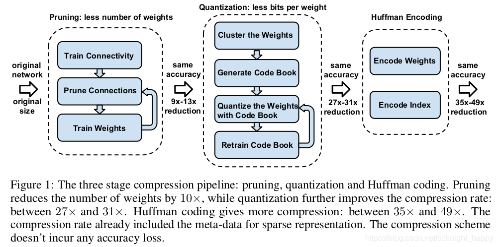

1.1 模型剪枝及稀疏矩阵的存储

模型剪枝就是作者的上篇文章的介绍内容：https://blog.csdn.net/cdknight_happy/article/details/110953977

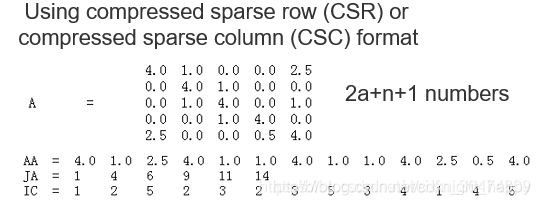
剪枝之后，大量的权重稀疏变为了0，矩阵变为了稀疏矩阵，可以采用CSR或CSC的方式进行稀疏矩阵的存储，将n * n的稀疏矩阵使用2a + n + 1个值进行表示，a表示非零元素的个数。

本节下面的内容参考：https://blog.csdn.net/weixin_36474809/article/details/80643784

稀疏权值矩阵的存储：比如我们这个稀疏的矩阵A里面，n×n的矩阵，里面大多数的值是零值，然后我们通过相应的存储稀疏矩阵的方式对这个矩阵进行存储。首先把所有的非零值存为AA，假设所有的非零值的元素的个数为a，然后把每一行第一个非零元素对应在AA的位置存为JA，最后一个数是所有非零元素的个数+1，所以JA中的元素就是行数n+1，然后把AA中每一个元素在原始矩阵中的列存为IC。所以我们把一个原始的n×n的稀疏矩阵存为2a+n+1个数字，达到了很好的存储压缩。复原时，通过JA可以将AA中所有元素对应的行恢复出来，IC又给出了所有非零元素的列，所以完全可以完成稀疏矩阵的恢复。

实现：scipy.sparse.csr_matrix和scipy.sparse.csr_matrix用于构建稀疏矩阵，当矩阵的行数小于列数时，使用scipy.sparse.csr_matrix，否则使用scipy.sparse.csc_matrix。

稀疏矩阵构建完成后，mat.data中存储所有非零元素的值，对应上面的AA；mat.indices中存储非零元素的在原始矩阵中的列号，对应上面的IC；mat.indptr中存储每一行第一个非零元素在AA中的位置，对应于上面的JA。

1.2 量化

量化的目的是减少每一个权重存储所占用的bit数。作者的做法是通过让多个连接共享相同的权重减少必须要存储的有效权重的数量。

权重共享如Fig. 3所示：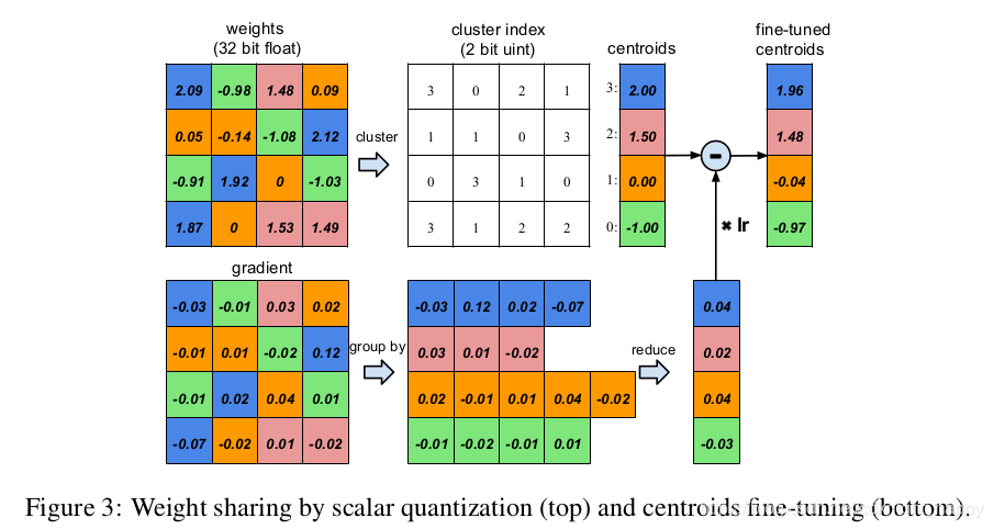
假设一个网络层包含四个输入神经元，四个输出神经元，权重矩阵大小为$4\times 4$，即上图左上图。权重矩阵中的16个系数按照其大小聚类成4类，按不同的颜色进行标识。所以，对于$4\times 4$的权重矩阵，我们只需要记录四个权重中心点的值及各个权重系数隶属的类别索引。进行权重更新时，属于同一类别的梯度信息被求和，乘以学习率对权重中心点进行更新。

假设量化后权重矩阵按照k个中心点进行聚类，那么编码索引矩阵需要${\log }_2(k)$个bit，需要存储k个存储聚类中心点。假设一个网络有n个连接，每个连接需要使用b个bit进行存储，那么量化前后的存储占用大小的比值，即压缩比，为：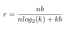

1.2.1 聚类中心点的选择

k-means聚类，需要人为设定聚类中心，聚类中心对最终的聚类结果有很大的影响。作者试验了三种聚类中心的设定方法，即随机选择、基于密度进行选择和线性选择。三种选择方式选出的聚类中心点如下图所示：

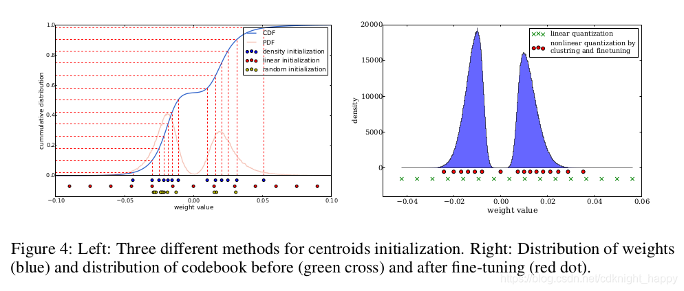
随机选择无需过多解释；基于密度进行选择是将y轴进行等距切分，将其映射到CDF(连续密度函数)上，交点再投影到x轴得到各中心点，如上左图中的蓝色点所示。线性选择就是把x轴进行等距离切分。在https://blog.csdn.net/cdknight_happy/article/details/110953977中，作者认为权重的幅值越大，其重要性越大，但是幅值大的权重占比很小。所以，对于随机选择和基于密度选择，很难选取某个幅值较大的权重作为其聚类中心点，所以聚类迭代过程中这些幅值很大的点会被遗弃掉，这部分较重要的权重被遗弃掉之后，对于模型的性能具有较大的负面影响。而对于线性选择，各个幅值范围的点都会被选出一个作为中心点，这样就避免了较大幅值被遗弃，压缩后可以取得更好的效果。下面的实验也佐证了这一观点。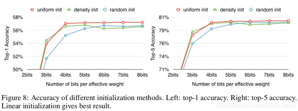

1.2.3 相对位置的存储

本节内容参考自：https://www.sohu.com/a/337658183_99979179

在量化完参数之后，作者没有存储类别索引的绝对值，而是存储类别索引的相对值，如Fig. 2所示，就是存储两个索引的差值。Fig. 2中用三个比特存相对的值，只要两个元素的距离小于8，直接在对应距离处存储，如果两个参数的距离大于8，我们就在第8个位置设置一个0值。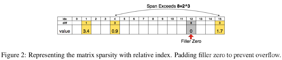

3bit可以存储的距离为8：

• 当间距小于8时：用3比特的值就可以恢复出相应的位置；
• 当间距大于8时：在第8个位置插入0值，然后用3bit的与插入的0值的差分位置恢复出相应的位置；
• 间距大于8的倍数时：每隔8个位置插入0值，与最后一个0值的3bit的差分位置恢复出位置

这样原始的存储方式：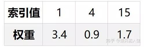

可以变成：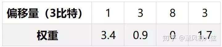

索引的存储从需要4个bit减少到了3个bit。

1.2.2 前向和后向过程

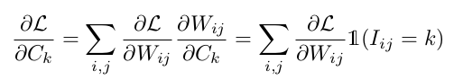
如Fig. 3所示，k-means聚类的每一个中心点都是一个共享权重。每一个连接按照其类别关联到某一个共享权重，必然存在多个连接关联同一个共享权重的情况。那么在反向传播时，关联到同一共享权重的所有连接对其的梯度应该进行累加进行参数更新。

用$L$表示损失，$W_{ij}$表示映射表中第i行第j列的元素，$W_{ij}$指定的类别中心为$I_{ij}$，对应第k个共享权重$C_k$。那么有：

1.3 Huffman编码

Huffman编码是一种可变长的无损压缩，核心思想是对于高频出现的样本给予更短的码字，从而最小化整个样本集的编码字长。可以参考https://blog.csdn.net/qq_36653505/article/details/81701181。

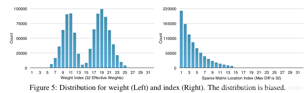
哈夫曼编码运用样本出现的概率来进行编码，只要不是均匀分布的，哈夫曼编码就能减少一定的冗余，比如在AlexNet中，如Fig. 5所示的相应的权值的分布直方图和权值参数的直方图，用哈夫曼编码可以减少20-30%的信息冗余。

作者在对模型进行剪枝和量化的基础上，进一步应用Huffman编码压缩总的存储空间。

2 实验

总的压缩效果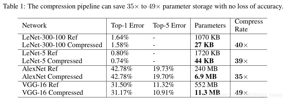
不降低模型准确率的情况下，压缩了35x到49x，赞

LeNet上各个压缩组件的作用：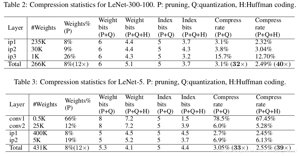
LeNet-300-100中，Q时，Weight bit = 6，Index bit=5，表示得到了$2^6=64$个聚类中心，索引矩阵按照相对存储方式使用5个bit存储，也就是最大相对位置偏差为32。LeNet-5中，Q时，卷积层Weight bit = 8，Index bit=5，表示得到了个$2^8=256$聚类中心，索引用5个bit存储相对位置；全连接层Weight bit = 5，Index bit=5，表示得到了个$2^5=32$聚类中心，索引用5个bit存储相对位置。

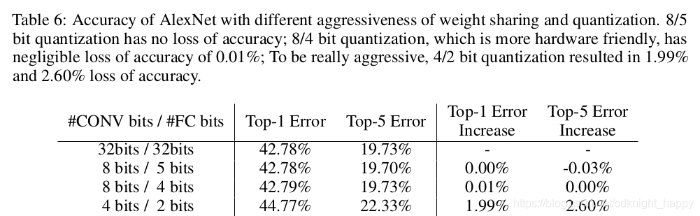
AlexNet 和 CGGNet：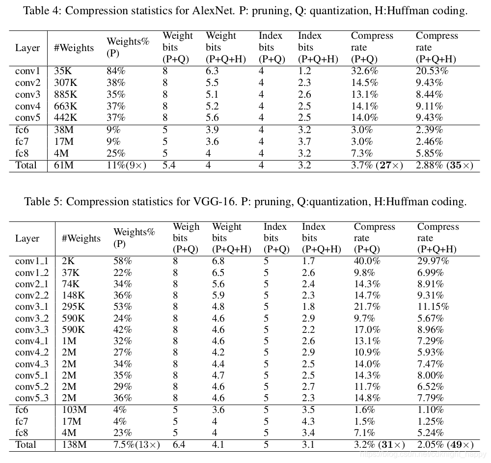
Q时，卷积层Weight bit = 8，Index bit=5，表示得到了个$2^8=256$聚类中心，索引用5个bit存储相对位置；全连接层Weight bit = 5，Index bit=5，表示得到了个$2^5=32$聚类中心，索引用5个bit存储相对位置。

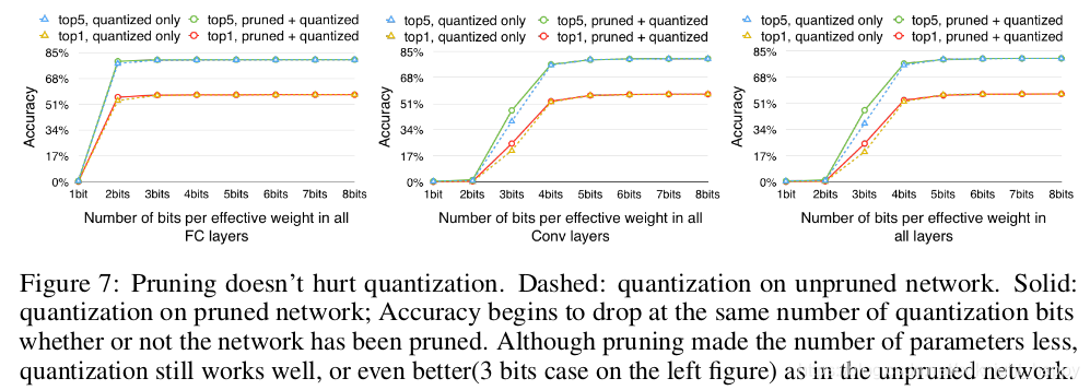
剪枝和量化互不干扰：

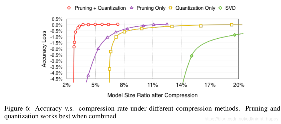先剪枝，权重矩阵变得稀疏，有效参数量大大减少。此时再进行量化，参数量少了，选取和只量化处理时同样多个聚类中心，量化误差更小，效果更好。

本文算法在不同类型设备上的加速效果和能耗对比：
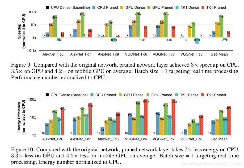测量加速效果和能耗时按照batchsize=1进行测量，模拟实时处理的情况。

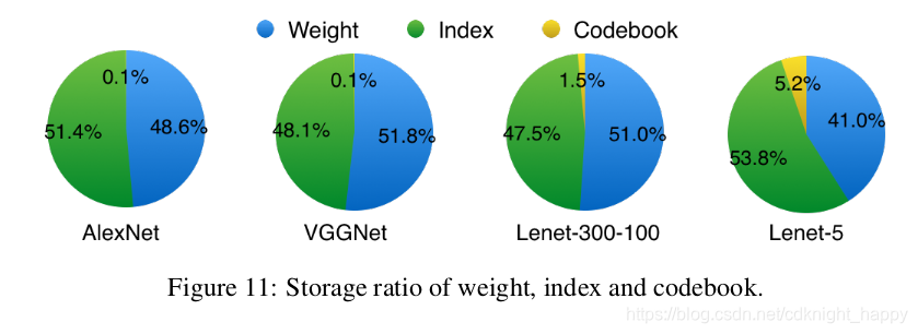
权重&索引&码本的比例：

对比其他模型压缩算法：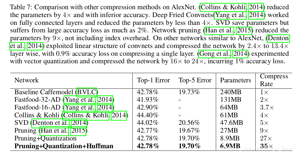

3 代码分析

3.1 剪枝代码

两种方式，一种是按照百分位决定阈值，一种是按照权重的标准差乘以一定的比例值决定阈值。

class PruningModule(Module):
    def prune_by_percentile(self, q=5.0, **kwargs):
        """
        Note:
             The pruning percentile is based on all layer's parameters concatenated
        Args:
            q (float): percentile in float
            **kwargs: may contain `cuda`
        """
        # Calculate percentile value
        alive_parameters = []
        for name, p in self.named_parameters():
            # We do not prune bias term
            if 'bias' in name or 'mask' in name:
                continue
            tensor = p.data.cpu().numpy()
            alive = tensor[np.nonzero(tensor)] # flattened array of nonzero values
            alive_parameters.append(alive)

        all_alives = np.concatenate(alive_parameters)
        percentile_value = np.percentile(abs(all_alives), q)
        print(f'Pruning with threshold : {percentile_value}')

        # Prune the weights and mask
        # Note that module here is the layer
        # ex) fc1, fc2, fc3
        for name, module in self.named_modules():
            if name in ['fc1', 'fc2', 'fc3']:
                module.prune(threshold=percentile_value)

    def prune_by_std(self, s=0.25):
        """
        Note that `s` is a quality parameter / sensitivity value according to the paper.
        According to Song Han's previous paper (Learning both Weights and Connections for Efficient Neural Networks),
        'The pruning threshold is chosen as a quality parameter multiplied by the standard deviation of a layer’s weights'

        I tried multiple values and empirically, 0.25 matches the paper's compression rate and number of parameters.
        Note : In the paper, the authors used different sensitivity values for different layers.
        """
        for name, module in self.named_modules():
            if name in ['fc1', 'fc2', 'fc3']:
                threshold = np.std(module.weight.data.cpu().numpy()) * s
                print(f'Pruning with threshold : {threshold} for layer {name}')
                module.prune(threshold)

###model.prune()
def prune(self, threshold):
    weight_dev = self.weight.device
    mask_dev = self.mask.device
    # Convert Tensors to numpy and calculate
    tensor = self.weight.data.cpu().numpy()
    mask = self.mask.data.cpu().numpy()
    new_mask = np.where(abs(tensor) < threshold, 0, mask)
    # Apply new weight and mask
    self.weight.data = torch.from_numpy(tensor * new_mask).to(weight_dev)
    self.mask.data = torch.from_numpy(new_mask).to(mask_dev)

3.2 量化代码

将剪枝后的矩阵转换为稀疏矩阵mat，按照线性初始化方法进行kmeans聚类，然后将原始权重的各元素值转换为其所隶属的聚类团簇的中心点的值。这里因为记录了前向过程中量化后的各权重值管理到哪个中心点，反向过程中也就针对该中心点进行了梯度累加，然后乘以学习率进行参数更新。总体上实现了本文中作者提出的量化思路。

import torch
import numpy as np
from sklearn.cluster import KMeans
from scipy.sparse import csc_matrix, csr_matrix


def apply_weight_sharing(model, bits=5):
    """
    Applies weight sharing to the given model
    """
    for module in model.children():
        dev = module.weight.device
        weight = module.weight.data.cpu().numpy()
        shape = weight.shape
        mat = csr_matrix(weight) if shape[0] < shape[1] else csc_matrix(weight)
        min_ = min(mat.data)
        max_ = max(mat.data)
        space = np.linspace(min_, max_, num=2**bits)
        kmeans = KMeans(n_clusters=len(space), init=space.reshape(-1,1), n_init=1, precompute_distances=True, algorithm="full")
        kmeans.fit(mat.data.reshape(-1,1))
        new_weight = kmeans.cluster_centers_[kmeans.labels_].reshape(-1)
        mat.data = new_weight
        module.weight.data = torch.from_numpy(mat.toarray()).to(dev)

3.3 huffman编码代码

对一个模型进行huffman编码的过程为，将各层的参数转换为稀疏矩阵进行存储，然后稀疏矩阵的data,index,indptr分别进行编码。在每类对象的huffman编码过程中，都是先计算各个数字出现的频率，使用heapq按照各样本出现的频率构建最小堆，然后按照https://blog.csdn.net/qq_36653505/article/details/81701181中介绍的思想进行huffman编码，最后存储各数据的huffman码字和总的codebook。这里同样给出了码字和codebook的读取、反编码的实现。

import os
from collections import defaultdict, namedtuple
from heapq import heappush, heappop, heapify
import struct
from pathlib import Path

import torch
import numpy as np
from scipy.sparse import csr_matrix, csc_matrix

Node = namedtuple('Node', 'freq value left right')
Node.__lt__ = lambda x, y: x.freq < y.freq

def huffman_encode(arr, prefix, save_dir='./'):
    """
    Encodes numpy array 'arr' and saves to `save_dir`
    The names of binary files are prefixed with `prefix`
    returns the number of bytes for the tree and the data after the compression
    """
    # Infer dtype
    dtype = str(arr.dtype)

    # Calculate frequency in arr
    freq_map = defaultdict(int)
    convert_map = {'float32':float, 'int32':int}
    for value in np.nditer(arr):
        value = convert_map[dtype](value)
        freq_map[value] += 1

    # Make heap
    heap = [Node(frequency, value, None, None) for value, frequency in freq_map.items()]
    heapify(heap)

    # Merge nodes
    while(len(heap) > 1):
        node1 = heappop(heap)
        node2 = heappop(heap)
        merged = Node(node1.freq + node2.freq, None, node1, node2)
        heappush(heap, merged)

    # Generate code value mapping
    value2code = {}

    def generate_code(node, code):
        if node is None:
            return
        if node.value is not None:
            value2code[node.value] = code
            return
        generate_code(node.left, code + '0')
        generate_code(node.right, code + '1')

    root = heappop(heap)
    generate_code(root, '')

    # Path to save location
    directory = Path(save_dir)

    # Dump data
    data_encoding = ''.join(value2code[convert_map[dtype](value)] for value in np.nditer(arr))
    datasize = dump(data_encoding, directory/f'{prefix}.bin')

    # Dump codebook (huffman tree)
    codebook_encoding = encode_huffman_tree(root, dtype)
    treesize = dump(codebook_encoding, directory/f'{prefix}_codebook.bin')

    return treesize, datasize


def huffman_decode(directory, prefix, dtype):
    """
    Decodes binary files from directory
    """
    directory = Path(directory)

    # Read the codebook
    codebook_encoding = load(directory/f'{prefix}_codebook.bin')
    root = decode_huffman_tree(codebook_encoding, dtype)

    # Read the data
    data_encoding = load(directory/f'{prefix}.bin')

    # Decode
    data = []
    ptr = root
    for bit in data_encoding:
        ptr = ptr.left if bit == '0' else ptr.right
        if ptr.value is not None: # Leaf node
            data.append(ptr.value)
            ptr = root

    return np.array(data, dtype=dtype)


# Logics to encode / decode huffman tree
# Referenced the idea from https://stackoverflow.com/questions/759707/efficient-way-of-storing-huffman-tree
def encode_huffman_tree(root, dtype):
    """
    Encodes a huffman tree to string of '0's and '1's
    """
    converter = {'float32':float2bitstr, 'int32':int2bitstr}
    code_list = []
    def encode_node(node):
        if node.value is not None: # node is leaf node
            code_list.append('1')
            lst = list(converter[dtype](node.value))
            code_list.extend(lst)
        else:
            code_list.append('0')
            encode_node(node.left)
            encode_node(node.right)
    encode_node(root)
    return ''.join(code_list)


def decode_huffman_tree(code_str, dtype):
    """
    Decodes a string of '0's and '1's and costructs a huffman tree
    """
    converter = {'float32':bitstr2float, 'int32':bitstr2int}
    idx = 0
    def decode_node():
        nonlocal idx
        info = code_str[idx]
        idx += 1
        if info == '1': # Leaf node
            value = converter[dtype](code_str[idx:idx+32])
            idx += 32
            return Node(0, value, None, None)
        else:
            left = decode_node()
            right = decode_node()
            return Node(0, None, left, right)

    return decode_node()



# My own dump / load logics
def dump(code_str, filename):
    """
    code_str : string of either '0' and '1' characters
    this function dumps to a file
    returns how many bytes are written
    """
    # Make header (1 byte) and add padding to the end
    # Files need to be byte aligned.
    # Therefore we add 1 byte as a header which indicates how many bits are padded to the end
    # This introduces minimum of 8 bits, maximum of 15 bits overhead
    num_of_padding = -len(code_str) % 8
    header = f"{num_of_padding:08b}"
    code_str = header + code_str + '0' * num_of_padding

    # Convert string to integers and to real bytes
    byte_arr = bytearray(int(code_str[i:i+8], 2) for i in range(0, len(code_str), 8))

    # Dump to a file
    with open(filename, 'wb') as f:
        f.write(byte_arr)
    return len(byte_arr)


def load(filename):
    """
    This function reads a file and makes a string of '0's and '1's
    """
    with open(filename, 'rb') as f:
        header = f.read(1)
        rest = f.read() # bytes
        code_str = ''.join(f'{byte:08b}' for byte in rest)
        offset = ord(header)
        if offset != 0:
            code_str = code_str[:-offset] # string of '0's and '1's
    return code_str


# Helper functions for converting between bit string and (float or int)
def float2bitstr(f):
    four_bytes = struct.pack('>f', f) # bytes
    return ''.join(f'{byte:08b}' for byte in four_bytes) # string of '0's and '1's

def bitstr2float(bitstr):
    byte_arr = bytearray(int(bitstr[i:i+8], 2) for i in range(0, len(bitstr), 8))
    return struct.unpack('>f', byte_arr)[0]

def int2bitstr(integer):
    four_bytes = struct.pack('>I', integer) # bytes
    return ''.join(f'{byte:08b}' for byte in four_bytes) # string of '0's and '1's

def bitstr2int(bitstr):
    byte_arr = bytearray(int(bitstr[i:i+8], 2) for i in range(0, len(bitstr), 8))
    return struct.unpack('>I', byte_arr)[0]


# Functions for calculating / reconstructing index diff
def calc_index_diff(indptr):
    return indptr[1:] - indptr[:-1]

def reconstruct_indptr(diff):
    return np.concatenate([[0], np.cumsum(diff)])


# Encode / Decode models
def huffman_encode_model(model, directory='encodings/'):
    os.makedirs(directory, exist_ok=True)
    original_total = 0
    compressed_total = 0
    print(f"{'Layer':<15} | {'original':>10} {'compressed':>10} {'improvement':>11} {'percent':>7}")
    print('-'*70)
    for name, param in model.named_parameters():
        if 'mask' in name:
            continue
        if 'weight' in name:
            weight = param.data.cpu().numpy()
            shape = weight.shape
            form = 'csr' if shape[0] < shape[1] else 'csc'
            mat = csr_matrix(weight) if shape[0] < shape[1] else csc_matrix(weight)

            # Encode
            t0, d0 = huffman_encode(mat.data, name+f'_{form}_data', directory)
            t1, d1 = huffman_encode(mat.indices, name+f'_{form}_indices', directory)
            t2, d2 = huffman_encode(calc_index_diff(mat.indptr), name+f'_{form}_indptr', directory)

            # Print statistics
            original = mat.data.nbytes + mat.indices.nbytes + mat.indptr.nbytes
            compressed = t0 + t1 + t2 + d0 + d1 + d2

            print(f"{name:<15} | {original:10} {compressed:10} {original / compressed:>10.2f}x {100 * compressed / original:>6.2f}%")
        else: # bias
            # Note that we do not huffman encode bias
            bias = param.data.cpu().numpy()
            bias.dump(f'{directory}/{name}')

            # Print statistics
            original = bias.nbytes
            compressed = original

            print(f"{name:<15} | {original:10} {compressed:10} {original / compressed:>10.2f}x {100 * compressed / original:>6.2f}%")
        original_total += original
        compressed_total += compressed

    print('-'*70)
    print(f"{'total':15} | {original_total:>10} {compressed_total:>10} {original_total / compressed_total:>10.2f}x {100 * compressed_total / original_total:>6.2f}%")


def huffman_decode_model(model, directory='encodings/'):
    for name, param in model.named_parameters():
        if 'mask' in name:
            continue
        if 'weight' in name:
            dev = param.device
            weight = param.data.cpu().numpy()
            shape = weight.shape
            form = 'csr' if shape[0] < shape[1] else 'csc'
            matrix = csr_matrix if shape[0] < shape[1] else csc_matrix

            # Decode data
            data = huffman_decode(directory, name+f'_{form}_data', dtype='float32')
            indices = huffman_decode(directory, name+f'_{form}_indices', dtype='int32')
            indptr = reconstruct_indptr(huffman_decode(directory, name+f'_{form}_indptr', dtype='int32'))

            # Construct matrix
            mat = matrix((data, indices, indptr), shape)

            # Insert to model
            param.data = torch.from_numpy(mat.toarray()).to(dev)
        else:
            dev = param.device
            bias = np.load(directory+'/'+name)
            param.data = torch.from_numpy(bias).to(dev)

##调用
huffman_encode_model(model)