目录

一、自定义二维卷积算子

二、自定义带步长和零填充的二维卷积算子

三、实现图像边缘检测

四、自定义卷积层算子和汇聚层算子

五、学习torch.nn.Conv2d()、torch.nn.MaxPool2d()；torch.nn.avg_pool2d()，简要介绍使用方法

1.torch.nn.Conv2d()：二维卷积层

2.torch.nn.MaxPool2d()：二维最大池化，降低尺寸，减少数据量。

3.torch.nn.avg_pool2d()：二维平均池化。

六、分别用自定义卷积算子和torch.nn.Conv2d()编程实现下面的卷积运算

附完整代码：

一、自定义二维卷积算子

代码如下：

# 自定义的卷积算子
class Conv2D(nn.Module):
    def __init__(self, kernel_size, w):
        super(Conv2D, self).__init__()
        w = torch.tensor(np.array(w, dtype='float32').reshape([kernel_size, kernel_size]))
        print("kernel:", w)
        self.weight = torch.nn.Parameter(w, requires_grad=True)

    def forward(self, X):
        u, v = self.weight.shape
        output = torch.zeros([X.shape[0], X.shape[1] - u + 1, X.shape[2] - v + 1])
        for i in range(output.shape[1]):
            for j in range(output.shape[2]):
                output[:, i, j] = torch.sum(X[:, i:i + u, j:j + v] * self.weight, axis=[1, 2])
        return output


# 使用二维卷积算子
# 随机构造一个二维输入矩阵
inputs = torch.as_tensor([[[1., 2., 3.],
                           [4., 5., 6.],
                           [7., 8., 9.]]])
w = [[1, 0],
     [1, 0]]
conv2d = Conv2D(kernel_size=2, w=w)
outputs = conv2d(inputs)
print("input: {}, \noutput: {}".format(inputs, outputs))

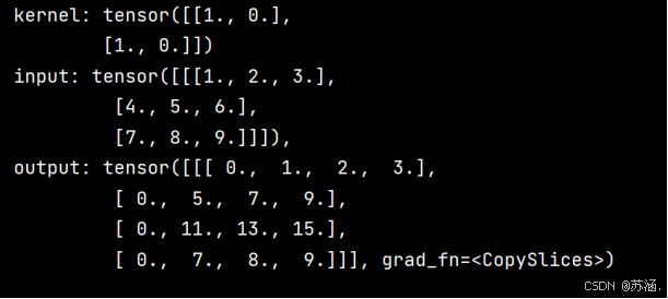
conv2d_2 = Conv2D_2(kernel_size=2, stride=1, padding=1, w=w)
outputs = conv2d_2(inputs)
print("input: {}, \noutput: {}".format(inputs, outputs))

运行结果如下：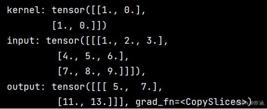
 

二、自定义带步长和零填充的二维卷积算子

代码如下：

# 自定义带步长和填充的卷积算子
class Conv2D_2(nn.Module):
    def __init__(self, kernel_size, stride, padding, w):
        super(Conv2D_2, self).__init__()
        w = torch.tensor(np.array(w, dtype='float32').reshape([kernel_size, kernel_size]))
        print("kernel:", w)
        self.weight = torch.nn.Parameter(w, requires_grad=True)
        self.stride = stride
        self.padding = padding

    def forward(self, X):
        new_X = torch.zeros([X.shape[0], X.shape[1] + 2 * self.padding, X.shape[2] + 2 * self.padding])
        new_X[:, self.padding:X.shape[1] + self.padding, self.padding:X.shape[2] + self.padding] = X
        u, v = self.weight.shape
        output_w = (new_X.shape[1] - u) // self.stride + 1
        output_h = (new_X.shape[2] - v) // self.stride + 1
        output = torch.zeros([X.shape[0], output_w, output_h])
        for i in range(0, output.shape[1]):
            for j in range(0, output.shape[2]):
                output[:, i, j] = torch.sum(
                    new_X[:, self.stride * i:self.stride * i + u, self.stride * j:self.stride * j + v] * self.weight,
                    axis=[1, 2])
        return output


# 使用二维卷积算子
# 随机构造一个二维输入矩阵
inputs = torch.as_tensor([[[1., 2., 3.],
                           [4., 5., 6.],
                           [7., 8., 9.]]])
w = [[1, 0],
     [1, 0]]
conv2d = Conv2D(kernel_size=2, w=w)
outputs = conv2d(inputs)
print("input: {}, \noutput: {}".format(inputs, outputs))

conv2d_2 = Conv2D_2(kernel_size=2, stride=1, padding=1, w=w)
outputs = conv2d_2(inputs)
print("input: {}, \noutput: {}".format(inputs, outputs))

运行结果如下：

 

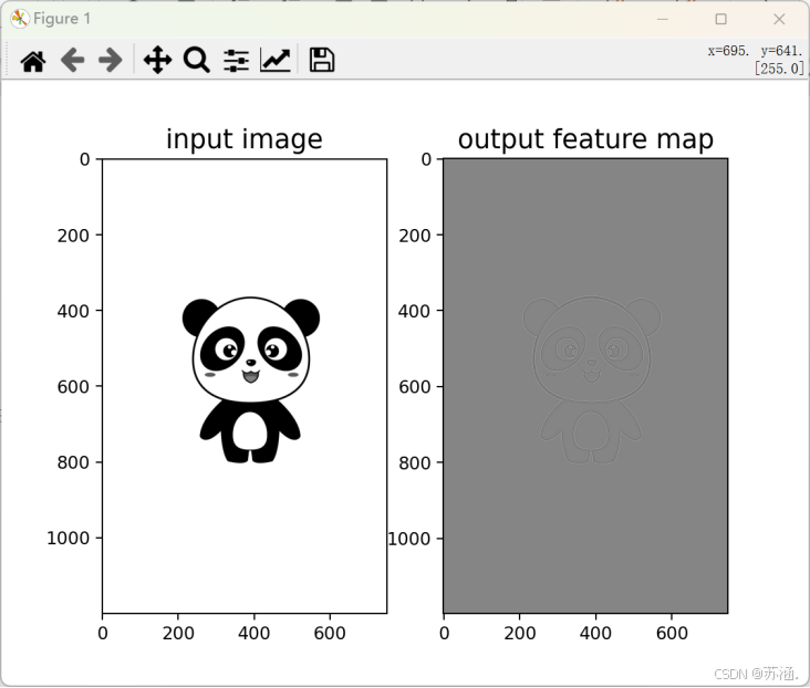
三、实现图像边缘检测

代码如下：

# 读取图片使用拉普拉斯算子进行边缘检测
w = [[-1, -1, -1],
     [-1, 8, -1],
     [-1, -1, -1]]
i = Image.open('panda.jpg').convert('L')
i = np.array(i, dtype='float32')
i = torch.from_numpy(i.reshape((i.shape[0], i.shape[1])))
# 创建卷积算子，卷积核大小为3x3，并使用上面的设置好的数值作为卷积核权重的初始化参数
time1 = time.time()
conv = Conv2D_2(kernel_size=3, stride=1, padding=0, w=w)
# 将读入的图片转化为float32类型的numpy.ndarray
inputs = np.array(i).astype('float32')
inputs = torch.as_tensor(inputs)
inputs = torch.unsqueeze(inputs, axis=0)
outputs = conv(inputs)
time2 = time.time()
print(outputs)
print("自定义算子运行时间:", time2-time1)

# 可视化结果
plt.subplot(121).set_title('input image', fontsize=15)
plt.imshow(i, cmap='gray')
plt.subplot(122).set_title('output feature map', fontsize=15)
plt.imshow(outputs.squeeze().detach().numpy(), cmap='gray')
plt.show()

# 比较与torch API运算结果
laplacian_kernel = torch.tensor([[-1, -1, -1],
                                 [-1, 8, -1],
                                 [-1, -1, -1]], dtype=torch.float32).unsqueeze(0).unsqueeze(0)  # 形状 (1, 1, 3, 3)
# bias_attr = torch.zeros([3, 1])
# bias_attr = torch.tensor(bias_attr, dtype=torch.float32)
time3 = time.time()
conv2d_torch = nn.Conv2d(in_channels=1, out_channels=1, kernel_size=3, padding=1, bias=False)
conv2d_torch.weight = torch.nn.Parameter(laplacian_kernel)
# 应用卷积操作
with torch.no_grad():
    edge_detected_image = conv(inputs)
# 转换回 numpy 并显示结果
edge_detected_image = edge_detected_image.squeeze().numpy()
outputs_torch = conv2d_torch(inputs)
time4 = time.time()
# 可视化结果
plt.subplot(121).set_title('input image', fontsize=15)
plt.imshow(i, cmap='gray')
plt.subplot(122).set_title('output feature map', fontsize=15)
plt.imshow(edge_detected_image, cmap='gray')
plt.show()
print("框架算子时间耗费:", time4 - time3)
print("===========================================================")

 运行结果如下：

 

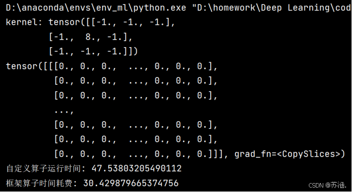
使用自定义算子和使用框架算子的运行结果一致，但是运行时间却大不相同，自定义的算子要慢很多，查找资料发现，nn.Conv2d 能高效处理批量数据，而自定义实现需要逐元素、逐通道进行卷积；同时，在自定义实现中，填充、切片和每次求和的操作都需要调用多次 torch 函数，而这些操作通常会导致额外的时间开销。 

四、自定义卷积层算子和汇聚层算子

代码如下：

# 自定义卷积层算子
class Conv2D_3(nn.Module):
    def __init__(self, in_channels, out_channels, kernel_size, stride=1, padding=0):
        super(Conv2D_3, self).__init__()
        # 创建卷积核
        weight = torch.zeros([out_channels, in_channels, kernel_size, kernel_size])
        weight = nn.init.constant(torch.tensor(weight, dtype=torch.float32), val=1.0)
        self.weight = torch.nn.Parameter(weight)
        # 创建偏置
        bias = torch.zeros([out_channels, 1])
        bias = nn.init.constant(torch.tensor(bias, dtype=torch.float32), val=0.0)  # 值可调整
        self.bias = torch.nn.Parameter(bias)
        # 步长
        self.stride = stride
        # 填充
        self.padding = padding
        # 输入通道数
        self.in_channels = in_channels
        # 输出通道数
        self.out_channels = out_channels

    # 基础卷积运算
    def single_forward(self, X, weight):
        # 零填充
        new_X = torch.zeros([X.shape[0], X.shape[1] + 2 * self.padding, X.shape[2] + 2 * self.padding])
        new_X[:, self.padding:X.shape[1] + self.padding, self.padding:X.shape[2] + self.padding] = X
        u, v = weight.shape
        output_w = (new_X.shape[1] - u) // self.stride + 1
        output_h = (new_X.shape[2] - v) // self.stride + 1
        output = torch.zeros([X.shape[0], output_w, output_h])
        for i in range(0, output.shape[1]):
            for j in range(0, output.shape[2]):
                output[:, i, j] = torch.sum(
                    new_X[:, self.stride * i:self.stride * i + u, self.stride * j:self.stride * j + v] * weight,
                    axis=[1, 2])
        return output

    def forward(self, inputs):
        feature_maps = []
        p = 0
        for w, b in zip(self.weight, self.bias):  # P个(w,b),每次计算一个特征图Zp
            multi_outs = []
            # 循环计算每个输入特征图对应的卷积结果
            for i in range(self.in_channels):
                single = self.single_forward(inputs[:, i, :, :], w[i])
                multi_outs.append(single)
                # print("Conv2D in_channels:",self.in_channels,"i:",i,"single:",single.shape)
            # 将所有卷积结果相加
            feature_map = torch.sum(torch.stack(multi_outs), axis=0) + b  # Zp
            feature_maps.append(feature_map)
            # print("Conv2D out_channels:",self.out_channels, "p:",p,"feature_map:",feature_map.shape)
            p += 1
        # 将所有Zp进行堆叠
        out = torch.stack(feature_maps, 1)
        return out


# 自定义汇聚层算子
class Pool2D(nn.Module):
    def __init__(self, size=(2, 2), mode='max', stride=1):
        super(Pool2D, self).__init__()
        # 汇聚方式
        self.mode = mode
        self.h, self.w = size
        self.stride = stride

    def forward(self, x):
        output_w = (x.shape[2] - self.w) // self.stride + 1
        output_h = (x.shape[3] - self.h) // self.stride + 1
        output = torch.zeros([x.shape[0], x.shape[1], output_w, output_h])
        # 汇聚
        for i in range(output.shape[2]):
            for j in range(output.shape[3]):
                # 最大汇聚
                if self.mode == 'max':
                    value_m = max(torch.max(
                        x[:, :, self.stride * i:self.stride * i + self.w, self.stride * j:self.stride * j + self.h],
                        axis=3).values[0][0])
                    output[:, :, i, j] = torch.tensor(value_m)
                    # 平均汇聚
                elif self.mode == 'avg':
                    output[:, :, i, j] = torch.mean(
                        x[:, :, self.stride * i:self.stride * i + self.w, self.stride * j:self.stride * j + self.h],
                    )

        return output


# =====================================================================
# 使用自定义卷积层算子
i = Image.open('panda.jpg').convert('L')
i = np.array(i, dtype='float32')
# inputs = torch.from_numpy(i.reshape((i.shape[0], i.shape[1])))
inputs = torch.tensor([[[[0.0, 1.0, 2.0], [3.0, 4.0, 5.0], [6.0, 7.0, 8.0]],
                        [[1.0, 2.0, 3.0], [4.0, 5.0, 6.0], [7.0, 8.0, 9.0]]]])
time1 = time.time()
conv2d = Conv2D_3(in_channels=2, out_channels=3, kernel_size=2)
print("inputs shape:", inputs.shape)
# 形状为(1, 2, 3, 3),一批，两通道，3*3大小
outputs = conv2d(inputs)
time2 = time.time()
print("Conv2D outputs shape:", outputs.shape)

# 比较与torch API运算结果
weight_attr = torch.ones([3, 2, 2, 2])
bias_attr = torch.zeros([3, 1])
bias_attr = torch.tensor(bias_attr, dtype=torch.float32)
time3 = time.time()
conv2d_torch = nn.Conv2d(in_channels=2, out_channels=3, kernel_size=2, bias=True)
conv2d_torch.weight = torch.nn.Parameter(weight_attr)
outputs_torch = conv2d_torch(inputs)
time4 = time.time()
# 自定义算子运算结果
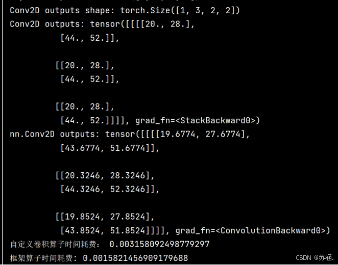
print('Conv2D outputs:', outputs)
# torch API运算结果
print('nn.Conv2D outputs:', outputs_torch)
print("自定义卷积算子时间耗费：", time2 - time1)
print("框架算子时间耗费:", time4 - time3)
print("=======================================================")

# ============================================================
inputs = torch.tensor([[[[1., 2., 3., 4.], [5., 6., 7., 8.], [9., 10., 11., 12.], [13., 14., 15., 16.]]]])
time1 = time.time()
pool2d = Pool2D(stride=2)
outputs = pool2d(inputs)
time2 = time.time()
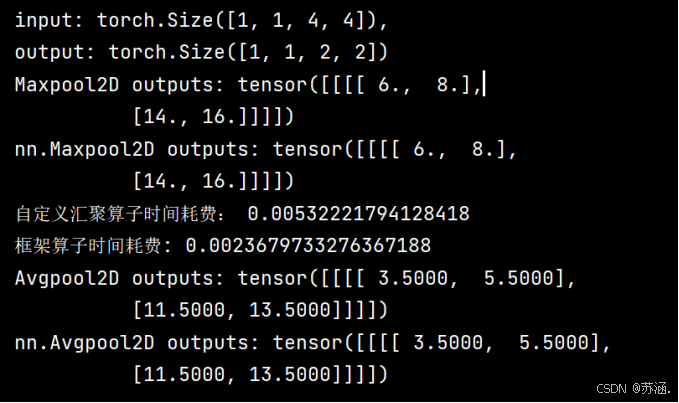
print("input: {}, \noutput: {}".format(inputs.shape, outputs.shape))
# 比较Maxpool2D和torch API运算结果
time3 = time.time()
maxpool2d_torch = nn.MaxPool2d(kernel_size=(2, 2), stride=2)
outputs_torch = maxpool2d_torch(inputs)
time4 = time.time()
# 自定义算子运算结果
print('Maxpool2D outputs:', outputs)
# torch API运算结果
print('nn.Maxpool2D outputs:', outputs_torch)
print("自定义汇聚算子时间耗费：", time2 - time1)
print("框架算子时间耗费:", time4 - time3)

# 比较Avgpool2D与torch API运算结果
avgpool2d_torch = nn.AvgPool2d(kernel_size=(2, 2), stride=2)
outputs_torch = avgpool2d_torch(inputs)
pool2d = Pool2D(mode='avg', stride=2)
outputs = pool2d(inputs)
# 自定义算子运算结果
print('Avgpool2D outputs:', outputs)
# torch API运算结果
print('nn.Avgpool2D outputs:', outputs_torch)

运行结果：

 

 

五、学习torch.nn.Conv2d()、torch.nn.MaxPool2d()；torch.nn.avg_pool2d()，简要介绍使用方法

1.torch.nn.Conv2d()：二维卷积层

使用方法：torch.nn.Conv2d(in_channels, out_channels, kernel_size, stride=1, padding=0, dilation=1, groups=1, bias=True)

前面几个分别是输入通道数、输出通道数、卷积核大小、步长、填充。

dilation用来控制卷积核元素之间的间距。dilation=1 表示卷积核的元素是相邻的，即不膨胀；当 dilation > 1 时，卷积核元素之间的间距会被拉大，相当于在卷积核内部插入“空洞”，因此也被称为空洞卷积。

groups用来控制输入通道与输出通道之间的连接方式。groups=1：标准卷积，每个输入通道与每个输出通道相连。groups=C：逐通道卷积，即每个输入通道仅与一个输出通道对应。

bias就是添加偏置项。

2.torch.nn.MaxPool2d()：二维最大池化，降低尺寸，减少数据量。

使用方法：torch.nn.MaxPool2d(kernel_size, stride=None, padding=0, dilation=1, return_indices=False, ceil_mode=False)

前面几个跟上面表示的一样。

return_indices：控制池化操作是否返回最大值所在的位置索引。
ceil_mode：控制池化区域是否采用上取整计算输出尺寸。默认是false，下取整。

3.torch.nn.avg_pool2d()：二维平均池化。

使用方法：torch.nn.functional.avg_pool2d(input, kernel_size, stride=None, padding=0, ceil_mode=False, count_include_pad=True)

count_include_pad：控制池化计算时是否将填充区域内的元素纳入平均值计算。

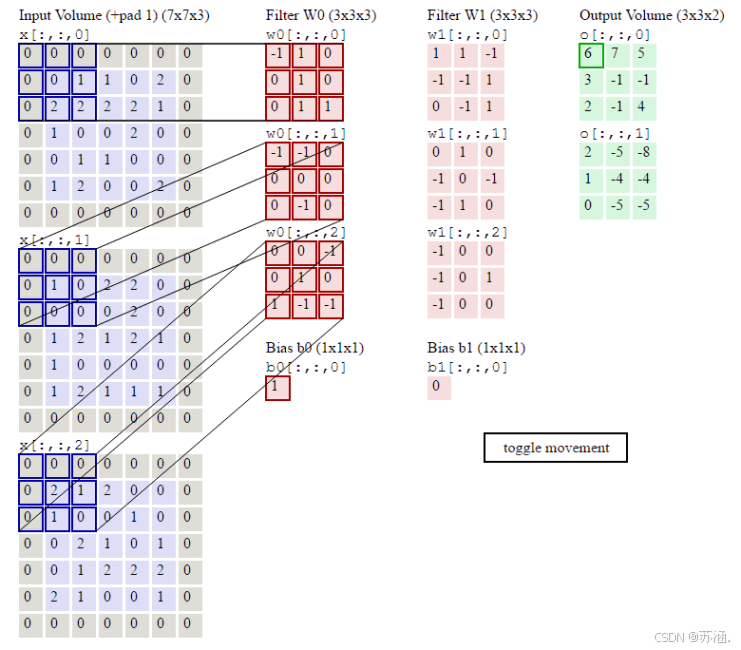
六、分别用自定义卷积算子和torch.nn.Conv2d()编程实现下面的卷积运算

代码如下：

import time

import torch
import torch.nn as nn


class Conv2D(nn.Module):
    def __init__(self, in_channels, out_channels, kernel_size, stride=1, padding=0, weight=[], bias=[]):
        super(Conv2D, self).__init__()
        # 创建偏置
        self.weight = nn.Parameter(weight)
        self.bias = nn.Parameter(bias)
        # 步长
        self.stride = stride
        # 补零
        self.padding = padding
        # 输入通道
        self.in_channels = in_channels
        # 输出通道
        self.out_channels = out_channels

    # 基础卷积运算
    def single_forward(self, X, weight):
        # 零填充
        new_X = torch.zeros([X.shape[0], X.shape[1] + 2 * self.padding, X.shape[2] + 2 * self.padding])
        new_X[:, self.padding:X.shape[1] + self.padding, self.padding:X.shape[2] + self.padding] = X
        u, v = weight.shape
        output_w = (new_X.shape[1] - u) // self.stride + 1
        output_h = (new_X.shape[2] - v) // self.stride + 1
        output = torch.zeros([X.shape[0], output_w, output_h])
        for i in range(0, output.shape[1]):
            for j in range(0, output.shape[2]):
                output[:, i, j] = torch.sum(
                    new_X[:, self.stride * i:self.stride * i + u, self.stride * j:self.stride * j + v] * weight,
                    axis=[1, 2])
        return output

    def forward(self, inputs):
        feature_maps = []
        p = 0
        for w, b in zip(self.weight, self.bias):
            multi_outs = []
            for i in range(self.in_channels):
                single = self.single_forward(inputs[:, i, :, :], w[i])
                multi_outs.append(single)
            feature_map = torch.sum(torch.stack(multi_outs), axis=0) + b  # Zp
            feature_maps.append(feature_map)
            p += 1
        out = torch.stack(feature_maps, 1)
        return out


# 分别使用自定义算子和torch.nn.Conv2d()实现三通道输入，两通道输出
# 使用自定义算子
inputs = torch.tensor([[[0.0, 1.0, 1.0, 0.0, 2.0], [2.0, 2.0, 2.0, 2.0, 1.0], [1.0, 0.0, 0.0, 2.0, 1.0],
                        [0.0, 1.0, 1.0, 0.0, 0.0], [1.0, 2.0, 0.0, 0.0, 2.0]],
                       [[1.0, 0.0, 2.0, 2.0, 0.0], [0.0, 0.0, 0.0, 2.0, 0.0], [1.0, 2.0, 1.0, 2.0, 1.0],
                        [1.0, 0.0, 0.0, 0.0, 0.0], [1.0, 2.0, 1.0, 1.0, 1.0]],
                       [[2.0, 1.0, 2.0, 0.0, 0.0], [1.0, 0.0, 0.0, 1.0, 0.0], [0.0, 2.0, 1.0, 0.0, 1.0],
                        [0.0, 1.0, 2.0, 2.0, 2.0], [2.0, 1.0, 0.0, 0.0, 1.0]]]).reshape([1, 3, 5, 5])
# 卷积层1
w1 = torch.tensor(
    [[[-1.0, 1.0, 0.0], [0.0, 1.0, 0.0], [0.0, 1.0, 1.0]], [[-1.0, -1.0, 0.0], [0.0, 0.0, 0.0], [0.0, -1.0, 0.0]],
     [[0.0, 0.0, -1.0], [0.0, 1.0, 0.0], [1.0, -1.0, -1.0]]], dtype=torch.float32).reshape([1, 3, 3, 3])
bias1 = torch.tensor(torch.ones([3, 1]))
time1 = time.time()
conv2d1 = Conv2D(in_channels=3, out_channels=1, kernel_size=3, stride=2, padding=1, weight=w1, bias=bias1)
outputs1 = conv2d1(inputs)
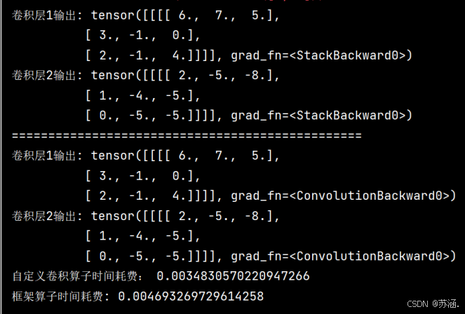
print("卷积层1输出:", outputs1)
# 卷积层2
w2 = torch.tensor(
    [[[1.0, 1.0, -1.0], [-1.0, -1.0, 1.0], [0.0, -1.0, 1.0]], [[0.0, 1.0, 0.0], [-1.0, 0.0, -1.0], [-1.0, 1.0, 0.0]],
     [[-1.0, 0.0, 0.0], [-1.0, 0.0, 1.0], [-1.0, 0.0, 0.0]]], dtype=torch.float32).reshape([1, 3, 3, 3])
bias2 = torch.tensor(torch.zeros([3, 1]))
conv2d2 = Conv2D(in_channels=3, out_channels=1, kernel_size=3, stride=2, padding=1, weight=w2, bias=bias2)
outputs2 = conv2d2(inputs)
time2 = time.time()
print("卷积层2输出:", outputs2)
print("================================================")

# 使用torch.nn.Conv2d()
time3 = time.time()
bias1 = torch.ones(1)  # 修改为一维向量，长度为 out_channels
bias2 = torch.zeros(1)  # 同样修改为一维向量，长度为 out_channels
conv2d_torch1 = nn.Conv2d(in_channels=3, out_channels=1, kernel_size=3, stride=2, padding=1, bias=True)
conv2d_torch1.weight = torch.nn.Parameter(w1)
conv2d_torch1.bias = torch.nn.Parameter(bias1)
outputs_torch1 = conv2d_torch1(inputs)
print("卷积层1输出:", outputs_torch1)
conv2d_torch2 = nn.Conv2d(in_channels=3, out_channels=1, kernel_size=3, stride=2, padding=1, bias=True)
conv2d_torch2.weight = torch.nn.Parameter(w2)
conv2d_torch2.bias = torch.nn.Parameter(bias2)
outputs_torch2 = conv2d_torch2(inputs)
print("卷积层2输出:", outputs_torch2)
time4 = time.time()
print("自定义卷积算子时间耗费：", time2 - time1)
print("框架算子时间耗费:", time4 - time3)

 运行结果：

补充知识点：

在卷积过程中，有时会希望跳过一些位置来降低计算的开销，将这一过程看作对标准交际运算输出的下采样。然后我看到下采样就想到了，那什么是上采样呢？最近读了一篇论文FCN，里面就利用到了上采样的知识。一般的卷积都是卷着卷着特征图就变小了，上采样就类似于宽卷积，通过插值等方法将图像扩大，进而使卷积后的图像可以恢复为原始图像大小，使输出的分割图与输入图像的像素位置一一对应。

拉普拉斯算子是一个大小为3×3的卷积核，中心元素值为8，其余元素值为-1.那为什么拉普拉斯算子的卷积核可以进行边缘检测呢？

拉普拉斯算子的这种结构使卷积核在处理图像的一个像素时，计算该像素与其邻域像素的差值之和，放大了像素值的差异。如果中心像素与周围像素的差异较大，卷积结果的值也会较大，因此边缘会被凸显出来。

 

附完整代码：

import torch
import torch.nn as nn
import torch.nn
import numpy as np
from PIL import Image
import time
from matplotlib import pyplot as plt
from torch.autograd import Variable


# 自定义的卷积算子
class Conv2D(nn.Module):
    def __init__(self, kernel_size, w):
        super(Conv2D, self).__init__()
        w = torch.tensor(np.array(w, dtype='float32').reshape([kernel_size, kernel_size]))
        print("kernel:", w)
        self.weight = torch.nn.Parameter(w, requires_grad=True)

    def forward(self, X):
        u, v = self.weight.shape
        output = torch.zeros([X.shape[0], X.shape[1] - u + 1, X.shape[2] - v + 1])
        for i in range(output.shape[1]):
            for j in range(output.shape[2]):
                output[:, i, j] = torch.sum(X[:, i:i + u, j:j + v] * self.weight, axis=[1, 2])
        return output


# 自定义带步长和填充的卷积算子
class Conv2D_2(nn.Module):
    def __init__(self, kernel_size, stride, padding, w):
        super(Conv2D_2, self).__init__()
        w = torch.tensor(np.array(w, dtype='float32').reshape([kernel_size, kernel_size]))
        print("kernel:", w)
        self.weight = torch.nn.Parameter(w, requires_grad=True)
        self.stride = stride
        self.padding = padding

    def forward(self, X):
        new_X = torch.zeros([X.shape[0], X.shape[1] + 2 * self.padding, X.shape[2] + 2 * self.padding])
        new_X[:, self.padding:X.shape[1] + self.padding, self.padding:X.shape[2] + self.padding] = X
        u, v = self.weight.shape
        output_w = (new_X.shape[1] - u) // self.stride + 1
        output_h = (new_X.shape[2] - v) // self.stride + 1
        output = torch.zeros([X.shape[0], output_w, output_h])
        for i in range(0, output.shape[1]):
            for j in range(0, output.shape[2]):
                output[:, i, j] = torch.sum(
                    new_X[:, self.stride * i:self.stride * i + u, self.stride * j:self.stride * j + v] * self.weight,
                    axis=[1, 2])
        return output


# 自定义卷积层算子
class Conv2D_3(nn.Module):
    def __init__(self, in_channels, out_channels, kernel_size, stride=1, padding=0):
        super(Conv2D_3, self).__init__()
        # 创建卷积核
        weight = torch.zeros([out_channels, in_channels, kernel_size, kernel_size])
        weight = nn.init.constant(torch.tensor(weight, dtype=torch.float32), val=1.0)
        self.weight = torch.nn.Parameter(weight)
        # 创建偏置
        bias = torch.zeros([out_channels, 1])
        bias = nn.init.constant(torch.tensor(bias, dtype=torch.float32), val=0.0)  # 值可调整
        self.bias = torch.nn.Parameter(bias)
        # 步长
        self.stride = stride
        # 填充
        self.padding = padding
        # 输入通道数
        self.in_channels = in_channels
        # 输出通道数
        self.out_channels = out_channels

    # 基础卷积运算
    def single_forward(self, X, weight):
        # 零填充
        new_X = torch.zeros([X.shape[0], X.shape[1] + 2 * self.padding, X.shape[2] + 2 * self.padding])
        new_X[:, self.padding:X.shape[1] + self.padding, self.padding:X.shape[2] + self.padding] = X
        u, v = weight.shape
        output_w = (new_X.shape[1] - u) // self.stride + 1
        output_h = (new_X.shape[2] - v) // self.stride + 1
        output = torch.zeros([X.shape[0], output_w, output_h])
        for i in range(0, output.shape[1]):
            for j in range(0, output.shape[2]):
                output[:, i, j] = torch.sum(
                    new_X[:, self.stride * i:self.stride * i + u, self.stride * j:self.stride * j + v] * weight,
                    axis=[1, 2])
        return output

    def forward(self, inputs):
        feature_maps = []
        p = 0
        for w, b in zip(self.weight, self.bias):  # P个(w,b),每次计算一个特征图Zp
            multi_outs = []
            # 循环计算每个输入特征图对应的卷积结果
            for i in range(self.in_channels):
                single = self.single_forward(inputs[:, i, :, :], w[i])
                multi_outs.append(single)
                # print("Conv2D in_channels:",self.in_channels,"i:",i,"single:",single.shape)
            # 将所有卷积结果相加
            feature_map = torch.sum(torch.stack(multi_outs), axis=0) + b  # Zp
            feature_maps.append(feature_map)
            # print("Conv2D out_channels:",self.out_channels, "p:",p,"feature_map:",feature_map.shape)
            p += 1
        # 将所有Zp进行堆叠
        out = torch.stack(feature_maps, 1)
        return out


# 自定义汇聚层算子
class Pool2D(nn.Module):
    def __init__(self, size=(2, 2), mode='max', stride=1):
        super(Pool2D, self).__init__()
        # 汇聚方式
        self.mode = mode
        self.h, self.w = size
        self.stride = stride

    def forward(self, x):
        output_w = (x.shape[2] - self.w) // self.stride + 1
        output_h = (x.shape[3] - self.h) // self.stride + 1
        output = torch.zeros([x.shape[0], x.shape[1], output_w, output_h])
        # 汇聚
        for i in range(output.shape[2]):
            for j in range(output.shape[3]):
                # 最大汇聚
                if self.mode == 'max':
                    value_m = max(torch.max(
                        x[:, :, self.stride * i:self.stride * i + self.w, self.stride * j:self.stride * j + self.h],
                        axis=3).values[0][0])
                    output[:, :, i, j] = torch.tensor(value_m)
                    # 平均汇聚
                elif self.mode == 'avg':
                    output[:, :, i, j] = torch.mean(
                        x[:, :, self.stride * i:self.stride * i + self.w, self.stride * j:self.stride * j + self.h],
                    )

        return output


# ==========================================================
# 使用二维卷积算子
# 随机构造一个二维输入矩阵
inputs = torch.as_tensor([[[1., 2., 3.],
                           [4., 5., 6.],
                           [7., 8., 9.]]])
w = [[1, 0],
     [1, 0]]
conv2d = Conv2D(kernel_size=2, w=w)
outputs = conv2d(inputs)
print("input: {}, \noutput: {}".format(inputs, outputs))

conv2d_2 = Conv2D_2(kernel_size=2, stride=1, padding=1, w=w)
outputs = conv2d_2(inputs)
print("input: {}, \noutput: {}".format(inputs, outputs))

# ===========================================================
# 读取图片使用拉普拉斯算子进行边缘检测
w = [[-1, -1, -1],
     [-1, 8, -1],
     [-1, -1, -1]]
i = Image.open('panda.jpg').convert('L')
i = np.array(i, dtype='float32')
i = torch.from_numpy(i.reshape((i.shape[0], i.shape[1])))
# 创建卷积算子，卷积核大小为3x3，并使用上面的设置好的数值作为卷积核权重的初始化参数
time1 = time.time()
conv = Conv2D_2(kernel_size=3, stride=1, padding=0, w=w)
# 将读入的图片转化为float32类型的numpy.ndarray
inputs = np.array(i).astype('float32')
inputs = torch.as_tensor(inputs)
inputs = torch.unsqueeze(inputs, axis=0)
outputs = conv(inputs)
time2 = time.time()
print(outputs)
print("自定义算子运行时间:", time2-time1)

# 可视化结果
plt.subplot(121).set_title('input image', fontsize=15)
plt.imshow(i, cmap='gray')
plt.subplot(122).set_title('output feature map', fontsize=15)
plt.imshow(outputs.squeeze().detach().numpy(), cmap='gray')
plt.show()

# 比较与torch API运算结果
laplacian_kernel = torch.tensor([[-1, -1, -1],
                                 [-1, 8, -1],
                                 [-1, -1, -1]], dtype=torch.float32).unsqueeze(0).unsqueeze(0)  # 形状 (1, 1, 3, 3)
# bias_attr = torch.zeros([3, 1])
# bias_attr = torch.tensor(bias_attr, dtype=torch.float32)
time3 = time.time()
conv2d_torch = nn.Conv2d(in_channels=1, out_channels=1, kernel_size=3, padding=1, bias=False)
conv2d_torch.weight = torch.nn.Parameter(laplacian_kernel)
# 应用卷积操作
with torch.no_grad():
    edge_detected_image = conv(inputs)
# 转换回 numpy 并显示结果
edge_detected_image = edge_detected_image.squeeze().numpy()
outputs_torch = conv2d_torch(inputs)
time4 = time.time()
# 可视化结果
plt.subplot(121).set_title('input image', fontsize=15)
plt.imshow(i, cmap='gray')
plt.subplot(122).set_title('output feature map', fontsize=15)
plt.imshow(edge_detected_image, cmap='gray')
plt.show()
print("框架算子时间耗费:", time4 - time3)
print("===========================================================")


# =====================================================================
# 使用自定义卷积层算子
i = Image.open('panda.jpg').convert('L')
i = np.array(i, dtype='float32')
# inputs = torch.from_numpy(i.reshape((i.shape[0], i.shape[1])))
inputs = torch.tensor([[[[0.0, 1.0, 2.0], [3.0, 4.0, 5.0], [6.0, 7.0, 8.0]],
                        [[1.0, 2.0, 3.0], [4.0, 5.0, 6.0], [7.0, 8.0, 9.0]]]])
time1 = time.time()
conv2d = Conv2D_3(in_channels=2, out_channels=3, kernel_size=2)
print("inputs shape:", inputs.shape)
# 形状为(1, 2, 3, 3),一批，两通道，3*3大小
outputs = conv2d(inputs)
time2 = time.time()
print("Conv2D outputs shape:", outputs.shape)

# 比较与torch API运算结果
weight_attr = torch.ones([3, 2, 2, 2])
bias_attr = torch.zeros([3, 1])
bias_attr = torch.tensor(bias_attr, dtype=torch.float32)
time3 = time.time()
conv2d_torch = nn.Conv2d(in_channels=2, out_channels=3, kernel_size=2, bias=True)
conv2d_torch.weight = torch.nn.Parameter(weight_attr)
outputs_torch = conv2d_torch(inputs)
time4 = time.time()
# 自定义算子运算结果
print('Conv2D outputs:', outputs)
# torch API运算结果
print('nn.Conv2D outputs:', outputs_torch)
print("自定义卷积算子时间耗费：", time2 - time1)
print("框架算子时间耗费:", time4 - time3)
print("=======================================================")

# ============================================================
inputs = torch.tensor([[[[1., 2., 3., 4.], [5., 6., 7., 8.], [9., 10., 11., 12.], [13., 14., 15., 16.]]]])
time1 = time.time()
pool2d = Pool2D(stride=2)
outputs = pool2d(inputs)
time2 = time.time()
print("input: {}, \noutput: {}".format(inputs.shape, outputs.shape))
# 比较Maxpool2D和torch API运算结果
time3 = time.time()
maxpool2d_torch = nn.MaxPool2d(kernel_size=(2, 2), stride=2)
outputs_torch = maxpool2d_torch(inputs)
time4 = time.time()
# 自定义算子运算结果
print('Maxpool2D outputs:', outputs)
# torch API运算结果
print('nn.Maxpool2D outputs:', outputs_torch)
print("自定义汇聚算子时间耗费：", time2 - time1)
print("框架算子时间耗费:", time4 - time3)

# 比较Avgpool2D与torch API运算结果
avgpool2d_torch = nn.AvgPool2d(kernel_size=(2, 2), stride=2)
outputs_torch = avgpool2d_torch(inputs)
pool2d = Pool2D(mode='avg', stride=2)
outputs = pool2d(inputs)
# 自定义算子运算结果
print('Avgpool2D outputs:', outputs)
# torch API运算结果
print('nn.Avgpool2D outputs:', outputs_torch)

# ===========================================================

 本次的分享就到这里，下次再见~