本文是机器学习sklearn的系列文章之一，下面是前面文章：

机器学习sklearn系列之决策树： 飘哥：机器学习sklearn系列之决策树

机器学习sklearn之随机森林（第一部分）：飘哥：机器学习sklearn之随机森林

机器学习sklearn之随机森林（第二部分）：飘哥：机器学习sklearn之随机森林（第二部分：随机森林的调参）

1. 实例：随机森林在乳腺癌数据上的调参

终于可以调参了，那我们就来调吧，终于可以开始调参了，我们使用乳腺癌数据来调参数，乳腺癌数据是sklearn自带的数据之一，它是自带的分类数据之一。

案例中，往往使用真实数据，为什么我们要使用sklearn自带的数据呢？因为真实数据在随机森林下的调参过程，往往非常缓慢。真实数据量大，维度高，在使用随机森林之前需要一系列的处理。原本，我为大家准备了kaggle上下载的辨别手写数字的数据，有4W多条记录700多个左右的特征，随机森林在这个辨别手写数字的数据上有非常好的表现，其调参案例也是非常经典，但是由于数据的维度太高，太过复杂，运行一次完整的网格搜索需要四五个小时。经典的泰坦尼克号数据，用来调参的话也是需要很长时间，因此我才选择sklearn当中自带的，结构相对清晰简单的数据来为大家做这个案例。大家感兴趣的话，可以直接到kaggle上进行下载，数据集名称是Digit Recognizer。（Kaggel是一个主要为开发商和数据科学家提供举办机器学习竞赛、托管数据库、编写和分享代码的平台。Digit Recognizer是平台上的一个练习项目。题目大意是做一个手写数字识别的分类任务，所给的数据有sample_submission.csv，test.csv和train.csv。sample_submission.csv给出了提交文件的例子（参考其格式），test.csv给出了需要进行分类的测试数据，train.csv给出了带有标签的训练数据。数据是28*28的图像，在提供的数据文件中以一个1*784的一维向量表示，csv文件中一行代表一张图片的向量表示。train.csv中每行开头有附加的一个标签，表示这张图片中写的数字。）

那我们接下来，就用乳腺癌数据，来看看我们的调参代码：

A. 导入需要的库

#导入乳腺癌数据集

from sklearn.datasets import load_breast_cancer

#导入随机森林分类器

from sklearn.ensemble import RandomForestClassifier

#选择模型搜索中的网格搜索

from sklearn.model_selection import GridSearchCV

#选择模型搜索中的交叉验证

from sklearn.model_selection import cross_val_score

#加入画图的库，Matplotlib是一个Python 2D绘图库

import matplotlib.pyplot as plt

import pandas as pd

import numpy as np

B. 导入数据集，探索数据

data = load_breast_cancer()

print(data)

输出结果：

{'data': array([[1.799e+01, 1.038e+01, 1.228e+02, ..., 2.654e-01, 4.601e-01,

1.189e-01],

[2.057e+01, 1.777e+01, 1.329e+02, ..., 1.860e-01, 2.750e-01,

8.902e-02],

[1.969e+01, 2.125e+01, 1.300e+02, ..., 2.430e-01, 3.613e-01,

8.758e-02],

...,

[1.660e+01, 2.808e+01, 1.083e+02, ..., 1.418e-01, 2.218e-01,

7.820e-02],

[2.060e+01, 2.933e+01, 1.401e+02, ..., 2.650e-01, 4.087e-01,

1.240e-01],

[7.760e+00, 2.454e+01, 4.792e+01, ..., 0.000e+00, 2.871e-01,

7.039e-02]]), 'target': array([0, 0, 0, 0, 0, 0, 0, 0, 0, 0, 0, 0, 0, 0, 0, 0, 0, 0, 0, 1, 1, 1,

0, 0, 0, 0, 0, 0, 0, 0, 0, 0, 0, 0, 0, 0, 0, 1, 0, 0, 0, 0, 0, 0,

0, 0, 1, 0, 1, 1, 1, 1, 1, 0, 0, 1, 0, 0, 1, 1, 1, 1, 0, 1, 0, 0,

1, 1, 1, 1, 0, 1, 0, 0, 1, 0, 1, 0, 0, 1, 1, 1, 0, 0, 1, 0, 0, 0,

1, 1, 1, 0, 1, 1, 0, 0, 1, 1, 1, 0, 0, 1, 1, 1, 1, 0, 1, 1, 0, 1,

1, 1, 1, 1, 1, 1, 1, 0, 0, 0, 1, 0, 0, 1, 1, 1, 0, 0, 1, 0, 1, 0,

0, 1, 0, 0, 1, 1, 0, 1, 1, 0, 1, 1, 1, 1, 0, 1, 1, 1, 1, 1, 1, 1,

1, 1, 0, 1, 1, 1, 1, 0, 0, 1, 0, 1, 1, 0, 0, 1, 1, 0, 0, 1, 1, 1,

1, 0, 1, 1, 0, 0, 0, 1, 0, 1, 0, 1, 1, 1, 0, 1, 1, 0, 0, 1, 0, 0,

0, 0, 1, 0, 0, 0, 1, 0, 1, 0, 1, 1, 0, 1, 0, 0, 0, 0, 1, 1, 0, 0,

1, 1, 1, 0, 1, 1, 1, 1, 1, 0, 0, 1, 1, 0, 1, 1, 0, 0, 1, 0, 1, 1,

1, 1, 0, 1, 1, 1, 1, 1, 0, 1, 0, 0, 0, 0, 0, 0, 0, 0, 0, 0, 0, 0,

0, 0, 1, 1, 1, 1, 1, 1, 0, 1, 0, 1, 1, 0, 1, 1, 0, 1, 0, 0, 1, 1,

1, 1, 1, 1, 1, 1, 1, 1, 1, 1, 1, 0, 1, 1, 0, 1, 0, 1, 1, 1, 1, 1,

1, 1, 1, 1, 1, 1, 1, 1, 1, 0, 1, 1, 1, 0, 1, 0, 1, 1, 1, 1, 0, 0,

0, 1, 1, 1, 1, 0, 1, 0, 1, 0, 1, 1, 1, 0, 1, 1, 1, 1, 1, 1, 1, 0,

0, 0, 1, 1, 1, 1, 1, 1, 1, 1, 1, 1, 1, 0, 0, 1, 0, 0, 0, 1, 0, 0,

1, 1, 1, 1, 1, 0, 1, 1, 1, 1, 1, 0, 1, 1, 1, 0, 1, 1, 0, 0, 1, 1,

1, 1, 1, 1, 0, 1, 1, 1, 1, 1, 1, 1, 0, 1, 1, 1, 1, 1, 0, 1, 1, 0,

1, 1, 1, 1, 1, 1, 1, 1, 1, 1, 1, 1, 0, 1, 0, 0, 1, 0, 1, 1, 1, 1,

1, 0, 1, 1, 0, 1, 0, 1, 1, 0, 1, 0, 1, 1, 1, 1, 1, 1, 1, 1, 0, 0,

1, 1, 1, 1, 1, 1, 0, 1, 1, 1, 1, 1, 1, 1, 1, 1, 1, 0, 1, 1, 1, 1,

1, 1, 1, 0, 1, 0, 1, 1, 0, 1, 1, 1, 1, 1, 0, 0, 1, 0, 1, 0, 1, 1,

1, 1, 1, 0, 1, 1, 0, 1, 0, 1, 0, 0, 1, 1, 1, 0, 1, 1, 1, 1, 1, 1,

1, 1, 1, 1, 1, 0, 1, 0, 0, 1, 1, 1, 1, 1, 1, 1, 1, 1, 1, 1, 1, 1,

1, 1, 1, 1, 1, 1, 1, 1, 1, 1, 1, 1, 0, 0, 0, 0, 0, 0, 1]), 'target_names': array(['malignant', 'benign'], dtype='<U9'), 'DESCR': '.. _breast_cancer_dataset:nnBreast cancer wisconsin (diagnostic) datasetn--------------------------------------------nn**Data Set Characteristics:**nn :Number of Instances: 569nn :Number of Attributes: 30 numeric, predictive attributes and the classnn :Attribute Information:n - radius (mean of distances from center to points on the perimeter)n - texture (standard deviation of gray-scale values)n - perimetern - arean - smoothness (local variation in radius lengths)n - compactness (perimeter^2 / area - 1.0)n - concavity (severity of concave portions of the contour)n - concave points (number of concave portions of the contour)n - symmetry n - fractal dimension ("coastline approximation" - 1)nn The mean, standard error, and "worst" or largest (mean of the threen largest values) of these features were computed for each image,n resulting in 30 features. For instance, field 3 is Mean Radius, fieldn 13 is Radius SE, field 23 is Worst Radius.nn - class:n - WDBC-Malignantn - WDBC-Benignnn :Summary Statistics:nn ===================================== ====== ======n Min Maxn ===================================== ====== ======n radius (mean): 6.981 28.11n texture (mean): 9.71 39.28n perimeter (mean): 43.79 188.5n area (mean): 143.5 2501.0n smoothness (mean): 0.053 0.163n compactness (mean): 0.019 0.345n concavity (mean): 0.0 0.427n concave points (mean): 0.0 0.201n symmetry (mean): 0.106 0.304n fractal dimension (mean): 0.05 0.097n radius (standard error): 0.112 2.873n texture (standard error): 0.36 4.885n perimeter (standard error): 0.757 21.98n area (standard error): 6.802 542.2n smoothness (standard error): 0.002 0.031n compactness (standard error): 0.002 0.135n concavity (standard error): 0.0 0.396n concave points (standard error): 0.0 0.053n symmetry (standard error): 0.008 0.079n fractal dimension (standard error): 0.001 0.03n radius (worst): 7.93 36.04n texture (worst): 12.02 49.54n perimeter (worst): 50.41 251.2n area (worst): 185.2 4254.0n smoothness (worst): 0.071 0.223n compactness (worst): 0.027 1.058n concavity (worst): 0.0 1.252n concave points (worst): 0.0 0.291n symmetry (worst): 0.156 0.664n fractal dimension (worst): 0.055 0.208n ===================================== ====== ======nn :Missing Attribute Values: Nonenn :Class Distribution: 212 - Malignant, 357 - Benignnn :Creator: Dr. William H. Wolberg, W. Nick Street, Olvi L. Mangasariannn :Donor: Nick Streetnn :Date: November, 1995nnThis is a copy of UCI ML Breast Cancer Wisconsin (Diagnostic) datasets.nhttps://goo.gl/U2Uwz2nnFeatures are computed from a digitized image of a fine needlenaspirate (FNA) of a breast mass. They describencharacteristics of the cell nuclei present in the image.nnSeparating plane described above was obtained usingnMultisurface Method-Tree (MSM-T) [K. P. Bennett, "Decision TreenConstruction Via Linear Programming." Proceedings of the 4thnMidwest Artificial Intelligence and Cognitive Science Society,npp. 97-101, 1992], a classification method which uses linearnprogramming to construct a decision tree. Relevant featuresnwere selected using an exhaustive search in the space of 1-4nfeatures and 1-3 separating planes.nnThe actual linear program used to obtain the separating planenin the 3-dimensional space is that described in:n[K. P. Bennett and O. L. Mangasarian: "Robust LinearnProgramming Discrimination of Two Linearly Inseparable Sets",nOptimization Methods and Software 1, 1992, 23-34].nnThis database is also available through the UW CS ftp server:nnftp http://ftp.cs.wisc.eduncd math-prog/cpo-dataset/machine-learn/WDBC/nn.. topic:: Referencesnn - W.N. Street, W.H. Wolberg and O.L. Mangasarian. Nuclear feature extraction n for breast tumor diagnosis. IS&T/SPIE 1993 International Symposium on n Electronic Imaging: Science and Technology, volume 1905, pages 861-870,n San Jose, CA, 1993.n - O.L. Mangasarian, W.N. Street and W.H. Wolberg. Breast cancer diagnosis and n prognosis via linear programming. Operations Research, 43(4), pages 570-577, n July-August 1995.n - W.H. Wolberg, W.N. Street, and O.L. Mangasarian. Machine learning techniquesn to diagnose breast cancer from fine-needle aspirates. Cancer Letters 77 (1994) n 163-171.', 'feature_names': array(['mean radius', 'mean texture', 'mean perimeter', 'mean area',

'mean smoothness', 'mean compactness', 'mean concavity',

'mean concave points', 'mean symmetry', 'mean fractal dimension',

'radius error', 'texture error', 'perimeter error', 'area error',

'smoothness error', 'compactness error', 'concavity error',

'concave points error', 'symmetry error',

'fractal dimension error', 'worst radius', 'worst texture',

'worst perimeter', 'worst area', 'worst smoothness',

'worst compactness', 'worst concavity', 'worst concave points',

'worst symmetry', 'worst fractal dimension'], dtype='<U23'), 'filename': '/anaconda3/lib/python3.7/site-packages/sklearn/datasets/data/breast_cancer.csv'}

#输出数据记录条数

print(data.data.shape)

输出结果（569条数据，30个特征，由于数据非常少，标签分类特别多，导致相应比值非常低，所以会预测到模型会过拟合，就是测试数据结果效果不佳）：

(569, 30)

#输出数据集标签

print(data.target)

输出结果（2分类数据，分布均匀）：

[0 0 0 0 0 0 0 0 0 0 0 0 0 0 0 0 0 0 0 1 1 1 0 0 0 0 0 0 0 0 0 0 0 0 0 0 0

1 0 0 0 0 0 0 0 0 1 0 1 1 1 1 1 0 0 1 0 0 1 1 1 1 0 1 0 0 1 1 1 1 0 1 0 0

1 0 1 0 0 1 1 1 0 0 1 0 0 0 1 1 1 0 1 1 0 0 1 1 1 0 0 1 1 1 1 0 1 1 0 1 1

1 1 1 1 1 1 0 0 0 1 0 0 1 1 1 0 0 1 0 1 0 0 1 0 0 1 1 0 1 1 0 1 1 1 1 0 1

1 1 1 1 1 1 1 1 0 1 1 1 1 0 0 1 0 1 1 0 0 1 1 0 0 1 1 1 1 0 1 1 0 0 0 1 0

1 0 1 1 1 0 1 1 0 0 1 0 0 0 0 1 0 0 0 1 0 1 0 1 1 0 1 0 0 0 0 1 1 0 0 1 1

1 0 1 1 1 1 1 0 0 1 1 0 1 1 0 0 1 0 1 1 1 1 0 1 1 1 1 1 0 1 0 0 0 0 0 0 0

0 0 0 0 0 0 0 1 1 1 1 1 1 0 1 0 1 1 0 1 1 0 1 0 0 1 1 1 1 1 1 1 1 1 1 1 1

1 0 1 1 0 1 0 1 1 1 1 1 1 1 1 1 1 1 1 1 1 0 1 1 1 0 1 0 1 1 1 1 0 0 0 1 1

1 1 0 1 0 1 0 1 1 1 0 1 1 1 1 1 1 1 0 0 0 1 1 1 1 1 1 1 1 1 1 1 0 0 1 0 0

0 1 0 0 1 1 1 1 1 0 1 1 1 1 1 0 1 1 1 0 1 1 0 0 1 1 1 1 1 1 0 1 1 1 1 1 1

1 0 1 1 1 1 1 0 1 1 0 1 1 1 1 1 1 1 1 1 1 1 1 0 1 0 0 1 0 1 1 1 1 1 0 1 1

0 1 0 1 1 0 1 0 1 1 1 1 1 1 1 1 0 0 1 1 1 1 1 1 0 1 1 1 1 1 1 1 1 1 1 0 1

1 1 1 1 1 1 0 1 0 1 1 0 1 1 1 1 1 0 0 1 0 1 0 1 1 1 1 1 0 1 1 0 1 0 1 0 0

1 1 1 0 1 1 1 1 1 1 1 1 1 1 1 0 1 0 0 1 1 1 1 1 1 1 1 1 1 1 1 1 1 1 1 1 1

1 1 1 1 1 1 1 0 0 0 0 0 0 1]

C. 简单建模

进行一次简单的建模，看看模型本身在数据集上的效果

#实例化，n_estimators=100，请帮我建立100棵树的随机森林，random_state=90，90是任意输入的，大家可以任意写入数值，这个数不会对我们的调参有太大的影响。只会生成不同的树。random_state输入的数字不一样，我们的结果不一样。

rfc = RandomForestClassifier(n_estimators=100,random_state=90)

#交叉验证，cv=10交叉验证10次，mean是每次结果求均值。

score_pre = cross_val_score(rfc,data.data,data.target,cv=10).mean()

print(score_pre)

输出结果：

0.9666925935528475

上面是我们还没有做任何调参数的情况下，数据的表现还不错，预测准确率已经达到了96.66%。在现实数据集上啊，这是基本上是不可能的。没有调参就上到96%的。我们前面提到kaggle的手写数字识别上面是有可能的。是80多的起调线，一直可以调到96%97%，大家有空可以自己去调下。

D. 调参第一步：无论如何先来调n_estimators

为什么我这里要使用学习曲线来调n_estimators可不可以用网络搜索可以当然可以用网络搜索了，我用学习曲线因为通过n_estimates值的变化得到模型的分数变化的趋势。我想观察n_estimators在什么取值开始变得平稳，是否一直推动模型整体准确率的上升等信息。我想找一个准确率不错的同时计算量又不是很大的点作为n_estimators的取值，如果每次建树都要建立几百棵，那运行会非常慢。

最开始先用学习曲线，可以帮助我们划定范围，我们n_estimators从0开始，每次取十个数作为一个阶段，也就是取1，11，21，31，41，为什么要这样？因为我们从零开始，estimate还是不能有0的，最小值是1，所以让他10棵树就选一个，一直到200，总共要建19次。

scorel = []
for i in range(0,200,10):
    rfc = RandomForestClassifier(n_estimators=i+1,
                                 n_jobs=-1,
                                 random_state=90)
    score = cross_val_score(rfc,data.data,data.target,cv=10).mean()
scorel.append(score)
#打印所有交叉验证中最高分值是多少，并打印它的索引下标。
print(max(scorel),(scorel.index(max(scorel))*10)+1)
plt.figure(figsize=[20,5])
plt.plot(range(1,201,10),scorel)
plt.show()
#注意运行时间会比较长，30-50秒之间

输出结果（结果中输出是第41个得到的最大值，你会看到比没有调整参数之前数字提升了。）：

0.9666925935528475

0.9684480598046841 41

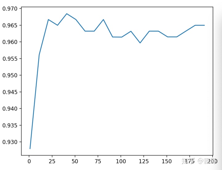
上图是画出来随着n_estimators的逐渐变大，然后模型展现出来的准确性，可以看到最开始在0~25之间的时候，这个准确性是这个非常稳定地往上升，后面开始逐渐波动，甚至有一些下降的趋势了，为什么?

到了后面之后estimators的作用就不再明显了，后面基本上就是持平甚至还有点下降，我们选择在25~50之间41作为下一步调参的指示。我在调的时候，我是问程序11， 21， 31， 41一直到201，你帮我选一个最大的，这并不代表说41就是局部中的最好结果了，下一步怎么样呢？我们在确定好了范围内进一步的来学习曲线。

E. 调参第二步：细化学习曲线

在确定好的范围内，进一步细化学习曲线。我已经知道这个模型在41左右的时候会有一个峰值，我想知道峰值是多少，那我就设定，请在35~45之间帮我训练几个模型，写出的代码和上面一样，

scorel = []

for i in range(35,45):

rfc = RandomForestClassifier(n_estimators=i,

n_jobs=-1,

random_state=90)

score = cross_val_score(rfc,data.data,data.target,cv=10).mean()

scorel.append(score)

print(max(scorel),([*range(35,45)][scorel.index(max(scorel))]))

plt.figure(figsize=[20,5])

plt.plot(range(35,45),scorel)

plt.show()

输出结果：

0.9666925935528475

0.9719568317345088 39

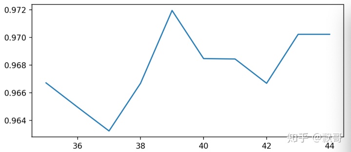
这一步其实是在上面的基础上细化。 我只是找出最好的值，当我把参数范围取小后，现在n_estimators最佳是39，可以看到准确率上升到0.9719568317345088，准确率提升了不少，n_estimators就选择39.

调整n_estimators的效果显著，模型的准确率立刻上升了0.005。接下来就进入网格搜索，我们将使用网格搜索对参数一个个进行调整。为什么我们不同时调整多个参数呢？原因有两个：1）同时调整多个参数会运行非常缓慢，在课堂上我们没有这么多的时间。2）同时调整多个参数，会让我们无法理解参数的组合是怎么得来的，所以即便网格搜索调出来的结果不好，我们也不知道从哪里去改。在这里，为了使用复杂度-泛化误差方法（方差-偏差方法），我们对参数进行一个个地调整。