fork了别人的项目，自己重新填写，我的代码如下

https://gitee.com/fakerlove/machine-learning/tree/master/code

代码原链接

2.吴恩达机器学习课程-作业2-逻辑回归

2.1 多变量逻辑回归

2.1.1 概念讲解

[外链图片转存失败,源站可能有防盗链机制,建议将图片保存下来直接上传(img-iPwl7gV7-1645517669338)(picture/v2-35393b75f51c81bb3c09774e76a7d91c_1440w.jpg)]

手稿如下，别人写的不是我的

[外链图片转存失败,源站可能有防盗链机制,建议将图片保存下来直接上传(img-mSbRM4Xd-1645517669346)(picture/04223814-734843250f1447d78a7e7c2e0f56e139.jpg)]

参考链接

https://zhuanlan.zhihu.com/p/36670444

Logistic Regression 虽然被称为回归，但其实际上是分类模型，并常用于二分类。Logistic Regression 因其简单、可并行化、可解释强深受工业界喜爱。

Logistic 回归的本质是：假设数据服从这个分布，然后使用极大似然估计做参数的估计。

2.1.2 题目介绍

在本部分的练习中，您将构建一个逻辑回归模型预测一个学生是否会被大学录取。假设你是一个大学部门的管理者，你想要根据每个申请人的两次考试的结果。

你有以前申请人的历史数据你可以用它作为逻辑回归的训练集。对于每一个培训例如，你有申请人的两次考试成绩和录取记录的决定。

你的任务是建立一个分类模型来估计申请人的录取概率基于这两门考试的分数。

2.1.3 数据介绍

34.62365962451697,78.0246928153624,0
30.28671076822607,43.89499752400101,0
35.84740876993872,72.90219802708364,0
60.18259938620976,86.30855209546826,1
79.0327360507101,75.3443764369103,1
45.08327747668339,56.3163717815305,0
61.10666453684766,96.51142588489624,1
75.02474556738889,46.55401354116538,1
76.09878670226257,87.42056971926803,1

第一列为第一门课程的成绩，第二列为第二门课程的成绩。第三行就是是否被录取，0就是没录取，1就是被录取

2.1.4 算法流程

1) 归一化

 def zeronorm(self, array):
        """
        Numpy数组的归一化处理--zero类型。把数据调到[-1,1]，平均值为0
        :param array: 需要归一化的数组
        :return:
        """
        std = array.std(axis=0)
        mean = array.mean(axis=0)
        data_rows = array.shape[0]
        data_cols = array.shape[1]
        t = np.empty((data_rows, data_cols))
        for i in range(data_cols):
            t[:, i] = (array[:, i] - mean[i]) / std[i]
        return t

2) 损失函数

本题采用sigmod函数。损失函数如下
$$\begin{gathered} L=-[ylog\hat{y}+(1-y)log(1-\hat{y})] \\ \hat{y}=\frac{1}{1+e^{-{\theta }^T\cdot x_b}}=\frac{1}{1+e^{-w^{T}x\cdot +b}} \end{gathered}$$
代码如下

def cost(self, X, y, theta):
        """
        计算损失函数值 $L=-[ylog\hat{y}+(1-y)log(1-\hat{y})]$

        :param X:
        :param y:
        :param theta:theta: 参数[b,w_1,w_2]
        :return:
        """
        hat_y = self.f(x=X, theta=theta)
        return np.mean((-y) * np.log(hat_y) - (1 - y) * np.log(1 - hat_y))
def sigmoid(self, z):
        """
        sigmoid函数实现了将结果从R转化到0-1，用来表示概率。实现sigmoid函数
        :param z: z值
        :return:
        """
        return 1 / (1 + np.exp(-z))

def f(self, x, theta):
        """
        计算函数值
        :param theta:
        :param x:
        :return:
        """
        # z=w_1x_1+w_2x_2+b，这里的theta=[b,w_1,w_2]
        z = x.dot(theta)
        return self.sigmoid(z)

3) 更新公式

$W\leftarrow W-\alpha X^T(\hat{Y}-Y)$

$b\leftarrow b-\alpha (\hat{Y}-Y)$

梯度公式$X^T(\hat{Y}-Y)$ 对应的代码

X.T.dot(hatY) / self.m

代码

    def gradient_descent(self, X, y, theta, iterations, alpha):
        """
        更新参数
        :param X: x,数据格式为[1,第一列成绩,第二列成绩],成绩是经过归一化后的
        :param y: y 是否被录取值
        :param theta: 参数[b,w_1,w_2]
        :param iterations: 迭代次数
        :param alpha: 步长
        :return: 参数,损失函数值
        """
        cost = []
        for i in range(iterations):
            hatY = self.f(x=X, theta=theta) - y
            # 更新参数
            theta -= alpha * X.T.dot(hatY) / self.m
            # 计算损失函数
            temp = self.cost(X=X, y=y, theta=theta)
            cost.append(temp)
        return theta, cost

4) 决策边界

如果样本只有两个特征，决策边界可以表示为

二维特征空间中，决策边界是一条理论上的直线，该直线是有线性模型的系数和截距决定的，并不一定有样本满足此条件\

${\theta }^{T}X={\theta }_0+{\theta }_1{x}_1+{\theta }_2{x}_2=0$​则该边界是一条直线，因为分类问题中特征空间的坐标轴都表示特征；

$x_2=\frac{-{\theta }_0-{\theta }_1{x}_1}{{\theta }_2}$​

每个地方表达式不一样，也可以表达如下

${\theta }_0=b,{\theta }_1=w_1,{\theta }_2=w_2$​​​

 # 因为进行了特征缩放，所以计算y时需要还原特征缩放,我还是没有搞懂为啥？？？？？。
x1 = np.arange(20, 110, 0.1)
std = self.data[:, 0:2].std(axis=0)
mean = self.data[:, 0:2].mean(axis=0)
x2 = mean[1] - std[1] * (theta[0] + theta[1] * (x1 - mean[0]) / std[0]) / theta[2]

2.1.5 代码介绍

import numpy as np
import matplotlib.pyplot as plt


class Logistic_Regression:

    def maxminnorm(self, array):
        """
        Numpy数组的归一化处理，把数据调到[0,1]
        :param array: 需要归一化的数组
        :return:
        """
        maxcols = array.max(axis=0)
        mincols = array.min(axis=0)
        data_rows = array.shape[0]
        data_cols = array.shape[1]
        t = np.empty((data_rows, data_cols))
        for i in range(data_cols):
            t[:, i] = (array[:, i] - mincols[i]) / (maxcols[i] - mincols[i])
        return t

    def meannorm(self, array):
        """
        Numpy数组的归一化处理--Mean类型。把数据调到[-1,1]，平均值为0
        :param array: 需要归一化的数组
        :return:
        """
        maxcols = array.max(axis=0)
        mincols = array.min(axis=0)
        meancols = array.mean(axis=0)
        data_rows = array.shape[0]
        data_cols = array.shape[1]
        t = np.empty((data_rows, data_cols))
        for i in range(data_cols):
            t[:, i] = (array[:, i] - meancols[i]) / (maxcols[i] - mincols[i])
        return t

    def zeronorm(self, array):
        """
        Numpy数组的归一化处理--zero类型。把数据调到[-1,1]，平均值为0
        :param array: 需要归一化的数组
        :return:
        """
        std = array.std(axis=0)
        mean = array.mean(axis=0)
        data_rows = array.shape[0]
        data_cols = array.shape[1]
        t = np.empty((data_rows, data_cols))
        for i in range(data_cols):
            t[:, i] = (array[:, i] - mean[i]) / std[i]
        return t

    def gradient_descent(self, X, y, theta, iterations, alpha):
        """
        更新参数
        :param X: x,数据格式为[1,第一列成绩,第二列成绩],成绩是经过归一化后的
        :param y: y 是否被录取值
        :param theta: 参数[b,w_1,w_2]
        :param iterations: 迭代次数
        :param alpha: 步长
        :return: 参数,损失函数值
        """
        cost = []
        for i in range(iterations):
            hatY = self.f(x=X, theta=theta) - y
            # 更新参数
            theta -= alpha * X.T.dot(hatY) / self.m
            # 计算损失函数
            temp = self.cost(X=X, y=y, theta=theta)
            cost.append(temp)
        return theta, cost

    def cost(self, X, y, theta):
        """
        计算损失函数值 $L=-[ylog\hat{y}+(1-y)log(1-\hat{y})]$

        :param X:
        :param y:
        :param theta:theta: 参数[b,w_1,w_2]
        :return:
        """
        hat_y = self.f(x=X, theta=theta)
        return np.mean((-y) * np.log(hat_y) - (1 - y) * np.log(1 - hat_y))

    def sigmoid(self, z):
        """
        sigmoid函数实现了将结果从R转化到0-1，用来表示概率。实现sigmoid函数
        :param z: z值
        :return:
        """
        return 1 / (1 + np.exp(-z))

    def f(self, x, theta):
        """
        计算函数值
        :param theta:
        :param x:
        :return:
        """
        # z=w_1x_1+w_2x_2+b，这里的theta=[b,w_1,w_2]
        z = x.dot(theta)
        return self.sigmoid(z)

    def __init__(self):
        """
        初始化数据
        """

        # 读取文件a.txt中的数据,分隔符为",",以double格式读取数据
        self.data = np.loadtxt('ex2data1.txt', delimiter=',', dtype=np.float64)
        # m设置行数
        self.m = self.data.shape[0]

        # X归一化后的数据.归一化使用zeronorm。
        # 多加了一列1 ，为了方便实现z= w_1x_1+w_2x_2+b,b乘以的正好是矩阵的1，就是b
        self.X = np.insert(self.zeronorm(self.data[:, 0:2]), 0, 1, axis=1)
        # self.X = np.insert(self.data[:, 0:2], 0, 1, axis=1)
        # y就是最后一列值
        self.y = self.data[:, 2]

        # 一共2*2，4个图，现在画第一个图

    # 计算x_2
    def x2(self, x1, theta):
        """
        x2()函数：求满足决策边界关系的直线的函数值；
        :param x1:
        :param w:
        :param b:
        :return:
        """
        w = theta[1:]
        b = theta[0]
        return (-w[0] * x1 - b) / w[1]

    def main(self):
        # 初始化参数
        alpha = 0.01  # 学习速率
        iterations = 10000  # 梯度下降的迭代轮数
        # 因为参数有3个z= w_1x_1+w_2x_2+b  theta=[b,w_1,w_2]
        theta = np.zeros(3)
        theta, cost = self.gradient_descent(self.X, self.y, theta, iterations, alpha)
        print("超平面为(%.3fx_1)+(%.3fx_2)+%.3f=0" % (theta[1], theta[2], theta[0]))
        # 绘制决策边界
        plt.subplot(2, 2, 1)
        plt.xlim((20, 110))
        plt.ylim((20, 110))
        plt.rcParams["font.sans-serif"] = ["SimHei"]
        plt.rcParams["axes.unicode_minus"] = False
        plt.title("逻辑回归来预测是否会被录取")  # 设置x
        plt.xlabel("第一次成绩")  # 设置x轴
        plt.ylabel("第二次成绩")  # 设置y轴
        x1 = np.arange(20, 110, 0.1)

        # 因为进行了特征缩放，所以计算y时需要还原特征缩放,我还是没有搞懂为啥？？？？？。
        std = self.data[:, 0:2].std(axis=0)
        mean = self.data[:, 0:2].mean(axis=0)
        x2 = mean[1] - std[1] * (theta[0] + theta[1] * (x1 - mean[0]) / std[0]) / theta[2]
        # x2 = self.x2(x1, theta)
        # print(x2)
        plt.plot(x1, x2, color='red', label="决策边界")
        # 绘制散点图
        # scatter绘制散点图
        for i in range(self.m):
            if self.data[i, 2] == 0:
                plt.scatter(self.data[i, 0], self.data[i, 1], marker='o', color="yellow", label='未被录取')
            else:
                plt.scatter(self.data[i, 0], self.data[i, 1], marker='+', color="black", label='被录取')

        # 绘制损失函数
        plt.subplot(2, 2, 4)
        plt.plot(range(iterations), cost)
        plt.show()


if __name__ == '__main__':
    print("========程序开始============")
    obj = Logistic_Regression()
    obj.main()
    print("========程序结束============")

结果如下

[外链图片转存失败,源站可能有防盗链机制,建议将图片保存下来直接上传(img-wwlUG8Z0-1645517669351)(picture/image-20211104223125347.png)]

2.2 逻辑回归的正则化

参考资料

https://blog.csdn.net/qq_37707218/article/details/108900715

2.2.1 题目介绍

在本部分的练习中，您将实现正则逻辑回归。预测制造工厂的微芯片是否通过质量保证(QA)。

在QA期间，每个芯片都要经过各种测试以确保它运行正常。假设你是工厂的产品经理，你有一些微芯的测试结果在两个不同的测试。

从这两个测试中，你想确定是否应该接受微芯片或拒绝。

为了帮助您做出决策，您有一个测试结果数据集在过去的微芯上，你可以从中建立一个逻辑回归模型。

2.2.2 数据格式

0.051267,0.69956,1
-0.092742,0.68494,1
-0.21371,0.69225,1
-0.375,0.50219,1
-0.51325,0.46564,1
-0.52477,0.2098,1
-0.39804,0.034357,1
-0.30588,-0.19225,1
0.016705,-0.40424,1
0.13191,-0.51389,1
0.38537,-0.56506,1
0.29896,0.61915,0
0.50634,0.75804,0
0.61578,0.7288,0
0.60426,0.59722,0
0.76555,0.50219,0
0.92684,0.3633,0
0.82316,0.27558,0
0.96141,0.085526,0

如图3所示，其中坐标轴是两个测试分数，以及正数(y = 1，被接受)和负数(y = 0，被拒绝)的例子如下所示不同的标记

[外链图片转存失败,源站可能有防盗链机制,建议将图片保存下来直接上传(img-HvmICDU5-1645517669353)(picture/image-20211105105712771.png)]

2.2.3 算法讲解

1) 非线性数据特征映射

那么如何使用逻辑回归算法得到非直线的决策边界呢？

特征只有两个，从数据中看，显然决策边界不能是线性的。因此需要使用通过构造高次多项式，形成非线性的决策边界。

我们回忆一下中学的数据知识——圆的表达式：

$x_1^2+x_2^2=r^2$​

这里需要实现对给定的$x_1$和$x_2$，通过构造1到n次多项式，形成新的特征。我们将特征映射到$x_1$和$x_2$​​​​的所有多项式项的六次方。

在本题目中，所谓特征映射就是将已知两个特征的各阶幂级数的乘积组合作为新的特征。

[外链图片转存失败,源站可能有防盗链机制,建议将图片保存下来直接上传(img-E6u7GBEx-1645517669355)(picture/20201002111712536.png)]

从2维变成28维。所以数组变成维数变成(118,28)

  def features_mapping(self, x1, x2, power):
        """
        两个特征进行最多power次特征映射
        :param x1:
        :param x2:
        :param power:
        :return:
        """

        m = len(x1)
        features = np.zeros((m, 1))
        for sum_power in range(power + 1):
            for x1_power in range(sum_power + 1):
                x2_power = sum_power - x1_power
                features = np.concatenate(
                    (features, (np.power(x1, x1_power) * np.power(x2, x2_power)).reshape(m, 1)),
                    axis=1)
        # np.delete
        # axis:=0按行删除，axis=1按列删除
        # array:需要处理的矩阵,
        # obj:需要处理的位置，比如要删除的第一行或者第一行和第二行
        # 删除第一列，因为第一列为0，np.zeros((m, 1))。没有任何用处
        return np.delete(features, 0, axis=1)

第二种–>特征映射，完全看自己选择

$h_{\theta }(x)={\theta }_0+{\theta }_1{x}_1+{\theta }_2{x}_2+\cdots$​

[外链图片转存失败,源站可能有防盗链机制,建议将图片保存下来直接上传(img-JUtiH8zt-1645517669358)(picture/cd913e35d1abb18ceb615959997b7f7b.JPEG)]

2) 正则化

在进行特征映以后，新增特征中就出现了很多原始特征的高阶项，而高阶项的出现则可能导致“过拟合”问题。

[外链图片转存失败,源站可能有防盗链机制,建议将图片保存下来直接上传(img-UifRxO3W-1645517669362)(picture/watermark,type_ZmFuZ3poZW5naGVpsadsadhuiasbcjdahsdj4.png)]

在逻辑回归中添加多项式项，从而得到不规则的决策边界，对非线性的数据进行很好的分类。添加多项式项之后，模型会变变得很复杂，非常容易出现过拟合，因此就需要使用正则化。

对损失函数增加$L_1$正则或$L_2$正则。可以引入一个新的参数 α来调节损失函数和正则项的权重，如：$J(\theta )+\alpha (L_1)$。

如果在损失函数前引入一个超参数$C$​​，即$C\cdot J(\theta )+L_1$​​，如果C越大，优化损失函数时越应该集中火力，将损失函数减小到最小；C非常小时，此时$L_1$​​和$L_2$​​的正则项就显得更加重要。其实损失函数前的参数**$C$​​**，作用相当于参数$\alpha$​​前的一个倒数。

在逻辑回归中，对模型正则化更喜欢使用**$C\cdot J(\theta )+L_1$**这种方式。
$$J(\theta )=\frac{1}{m}\sum _{i=1}^m[-ylog(\hat{y})-(1-y)log(1-\hat{y})]+\frac{\lambda }{2m}\sum _{j=1}^n{\theta }_j^2$$
上图中，最后的那一项即为“惩罚项”，其中的$\lambda$为正则化参数，它代表了“惩罚力度”。

因为在很多例子中，我们实现无法事先知道哪一项是高阶项，因此只能对除theta0之外的所有theta进行无差别惩罚（在假设函数中，theta0是与1相乘的，因此对theta0惩罚作用不大）。

因为惩罚项正是与各项相乘的参数组成的，在迭代中，代价函数值要想尽量小即必须使参数尽量小，这样一来也就减弱了高阶项对假设函数的影响，防止过拟合。

因为代价函数发生了变化，，因此其偏导随之变化，
$$\frac{\partial J(\theta )}{\partial {\theta }_j}=(\frac{1}{m}\sum _{i=1}^m(\hat{y}-y)x_j^{(i)})+\frac{\lambda }{m}{\theta }_j,forj\ge 1$$

    def cost(self, theta, X, y, l):
        """
        计算损失函数
        :param theta: 参数21个
        :param X: 映射后的X
        :param y:
        :param l: 为正则化参数，它代表了“惩罚力度”
        :return:
        """
        m = X.shape[0]
        hat_y = self.f(x=X, theta=theta)
        part1 = np.mean(-y * np.log(hat_y) - (1 - y) * np.log(1 - hat_y))
        part2 = (l / (2 * m)) * np.sum(np.delete((theta * theta), 0, axis=0))
        return part1 + part2

    def gradient(self, theta, X, y, l):
        """
        计算梯度
        :param theta: 带求参数
        :param X:
        :param y:
        :param l: 为正则化参数，它代表了“惩罚力度”
        :return:
        """
        m = self.m
        hat_y = self.f(x=X, theta=theta)
        part1 = X.T.dot(hat_y - y) / m
        part2 = (l / m) * theta
        part2[0] = 0
        return part1 + part2

2.2.4 代码讲解

参考链接

https://blog.csdn.net/qq_37707218/article/details/108900715
https://blog.csdn.net/m0_46297891/article/details/106322617

所有代码如下

import numpy as np
import matplotlib.pyplot as plt
from sklearn.metrics import classification_report


class Logistic_Regression:

    def cost(self, theta, X, y, l):
        """
        计算损失函数
        :param theta: 参数21个
        :param X: 映射后的X
        :param y:
        :param l: 为正则化参数，它代表了“惩罚力度”
        :return:
        """
        m = X.shape[0]
        hat_y = self.f(x=X, theta=theta)
        part1 = np.mean(-y * np.log(hat_y) - (1 - y) * np.log(1 - hat_y))
        part2 = (l / (2 * m)) * np.sum(np.delete((theta * theta), 0, axis=0))
        return part1 + part2

    def gradient(self, theta, X, y, l):
        """
        计算梯度
        :param theta: 带求参数
        :param X:
        :param y:
        :param l: 为正则化参数，它代表了“惩罚力度”
        :return:
        """
        m = self.m
        hat_y = self.f(x=X, theta=theta)
        part1 = X.T.dot(hat_y - y) / m
        part2 = (l / m) * theta
        part2[0] = 0
        return part1 + part2

    def sigmoid(self, z):
        """
        sigmoid函数实现了将结果从R转化到0-1，用来表示概率。实现sigmoid函数
        :param z: z值
        :return:
        """
        return 1 / (1 + np.exp(-z))

    def f(self, x, theta):
        """
        计算函数值
        :param theta:
        :param x:
        :return:
        """
        # z=w_1x_1+w_2x_2+b，这里的theta=[b,w_1,w_2]
        z = x.dot(theta)
        return self.sigmoid(z)

    def features_mapping(self, x1, x2, power):
        """
        两个特征进行最多power次特征映射
        :param x1:
        :param x2:
        :param power:
        :return:
        """
        m = len(x1)
        features = np.zeros((m, 1))
        for sum_power in range(power + 1):
            for x1_power in range(sum_power + 1):
                x2_power = sum_power - x1_power
                features = np.concatenate(
                    (features, (np.power(x1, x1_power) * np.power(x2, x2_power)).reshape(m, 1)),
                    axis=1)
        # np.delete
        # axis:=0按行删除，axis=1按列删除
        # array:需要处理的矩阵,
        # obj:需要处理的位置，比如要删除的第一行或者第一行和第二行
        # 删除第一列，因为第一列为0，np.zeros((m, 1))。没有任何用处
        return np.delete(features, 0, axis=1)

    def gradient_descent(self, X, y, theta, iterations, alpha, l):
        """
        更新参数，
        :param X:
        :param y:
        :param theta:
        :param iterations:
        :param alpha:
        :param l:
        :return:
        """
        cost = []
        for i in range(iterations):
            # 更新参数
            theta -= alpha * self.gradient(theta, X, y, l)
            # 计算损失函数值
            temp = self.cost(theta, X, y, l)
            cost.append(temp)
        return theta, cost

    def separate_dataset(self, data):
        """
        分离数据
        :param data:
        :return:
        """
        admit = np.empty(shape=(0, 2))
        not_admit = np.empty(shape=(0, 2))
        for i in range(self.m):
            if data[i, 2] == 0:
                not_admit = np.insert(arr=not_admit, obj=0, values=np.array([data[i, 0:2]]), axis=0)
            else:
                admit = np.insert(arr=admit, obj=0, values=np.array([data[i, 0:2]]), axis=0)
        return admit, not_admit

    def main(self):
        # 初始化参数
        alpha = 0.01  # 学习速率
        iterations = 10000  # 梯度下降的迭代轮数
        l = 1  # lambda 惩罚力度

        theta = np.zeros(self.features.shape[-1])
        theta, cost = self.gradient_descent(self.features, self.y, theta, iterations, alpha, l)
        # 绘制决策边界
        plt.rcParams["font.sans-serif"] = ["SimHei"]
        plt.rcParams["axes.unicode_minus"] = False
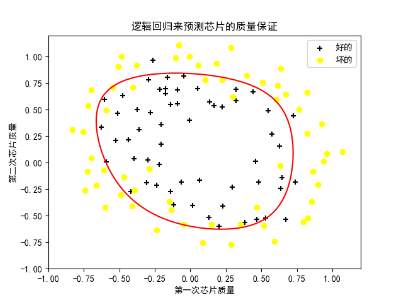
        plt.title("逻辑回归来预测芯片的质量保证")  # 设置x
        plt.xlabel("第一次芯片质量")  # 设置x轴
        plt.ylabel("第二次芯片质量")  # 设置y轴

        # 绘制散点图
        admit, not_admit = self.separate_dataset(data=self.data)
        plt.scatter(admit[:, 0], admit[:, 1], marker='+', color="black", label='好的')
        plt.scatter(not_admit[:, 0], not_admit[:, 1], marker='o', color="yellow", label='坏的')

        # 画出决策边界
        x = np.linspace(-1, 1.2, 100)
        x1, x2 = np.meshgrid(x, x)
        z = self.features_mapping(x1.ravel(), x2.ravel(), 6)
        z = z.dot(theta).reshape(x1.shape)
        plt.contour(x1, x2, z, 0, colors=['r'])
        plt.legend(loc='upper right')
        plt.show()

        # 打印这个函数的好坏
        print(classification_report(self.y, self.predict(theta, self.features)))

    def predict(self, theta, X):
        """
        训练完数据后，进行预测
        :param theta: 参数值
        :param X:
        :return:
        """
        return [1 if i > 0.5 else 0 for i in self.f(X, theta)]

    def __init__(self):
        """
        初始化数据
        """

        # 读取文件a.txt中的数据,分隔符为",",以double格式读取数据
        self.data = np.loadtxt('ex2data2.txt', delimiter=',', dtype=np.float64)

        # m设置行数
        self.m = self.data.shape[0]
        # 进行特征缩放
        self.features = self.features_mapping(self.data[..., 0], self.data[..., 1], 6)

        # y就是最后一列值
        self.y = self.data[:, 2]
        # 一共2*2，4个图，现在画第一个图


if __name__ == '__main__':
    print("========程序开始============")
    obj = Logistic_Regression()
    obj.main()
    print("========程序结束============")
import numpy as np
import matplotlib.pyplot as plt
from sklearn.metrics import classification_report


class Logistic_Regression:

    def cost(self, theta, X, y, l):
        """
        计算损失函数
        :param theta: 参数21个
        :param X: 映射后的X
        :param y:
        :param l: 为正则化参数，它代表了“惩罚力度”
        :return:
        """
        m = X.shape[0]
        hat_y = self.f(x=X, theta=theta)
        part1 = np.mean(-y * np.log(hat_y) - (1 - y) * np.log(1 - hat_y))
        part2 = (l / (2 * m)) * np.sum(np.delete((theta * theta), 0, axis=0))
        return part1 + part2

    def gradient(self, theta, X, y, l):
        """
        计算梯度
        :param theta: 带求参数
        :param X:
        :param y:
        :param l: 为正则化参数，它代表了“惩罚力度”
        :return:
        """
        m = self.m
        hat_y = self.f(x=X, theta=theta)
        part1 = X.T.dot(hat_y - y) / m
        part2 = (l / m) * theta
        part2[0] = 0
        return part1 + part2

    def sigmoid(self, z):
        """
        sigmoid函数实现了将结果从R转化到0-1，用来表示概率。实现sigmoid函数
        :param z: z值
        :return:
        """
        return 1 / (1 + np.exp(-z))

    def f(self, x, theta):
        """
        计算函数值
        :param theta:
        :param x:
        :return:
        """
        # z=w_1x_1+w_2x_2+b，这里的theta=[b,w_1,w_2]
        z = x.dot(theta)
        return self.sigmoid(z)

    def features_mapping(self, x1, x2, power):
        """
        两个特征进行最多power次特征映射
        :param x1:
        :param x2:
        :param power:
        :return:
        """
        m = len(x1)
        features = np.zeros((m, 1))
        for sum_power in range(power + 1):
            for x1_power in range(sum_power + 1):
                x2_power = sum_power - x1_power
                features = np.concatenate(
                    (features, (np.power(x1, x1_power) * np.power(x2, x2_power)).reshape(m, 1)),
                    axis=1)
        # np.delete
        # axis:=0按行删除，axis=1按列删除
        # array:需要处理的矩阵,
        # obj:需要处理的位置，比如要删除的第一行或者第一行和第二行
        # 删除第一列，因为第一列为0，np.zeros((m, 1))。没有任何用处
        return np.delete(features, 0, axis=1)

    def gradient_descent(self, X, y, theta, iterations, alpha, l):
        """
        更新参数，
        :param X:
        :param y:
        :param theta:
        :param iterations:
        :param alpha:
        :param l:
        :return:
        """
        cost = []
        for i in range(iterations):
            # 更新参数
            theta -= alpha * self.gradient(theta, X, y, l)
            # 计算损失函数值
            temp = self.cost(theta, X, y, l)
            cost.append(temp)
        return theta, cost

    def separate_dataset(self, data):
        """
        分离数据
        :param data:
        :return:
        """
        admit = np.empty(shape=(0, 2))
        not_admit = np.empty(shape=(0, 2))
        for i in range(self.m):
            if data[i, 2] == 0:
                not_admit = np.insert(arr=not_admit, obj=0, values=np.array([data[i, 0:2]]), axis=0)
            else:
                admit = np.insert(arr=admit, obj=0, values=np.array([data[i, 0:2]]), axis=0)
        return admit, not_admit

    def main(self):
        # 初始化参数
        alpha = 0.01  # 学习速率
        iterations = 10000  # 梯度下降的迭代轮数
        l = 1  # lambda 惩罚力度

        theta = np.zeros(self.features.shape[-1])
        theta, cost = self.gradient_descent(self.features, self.y, theta, iterations, alpha, l)
        # 绘制决策边界
        plt.rcParams["font.sans-serif"] = ["SimHei"]
        plt.rcParams["axes.unicode_minus"] = False
        plt.title("逻辑回归来预测芯片的质量保证")  # 设置x
        plt.xlabel("第一次芯片质量")  # 设置x轴
        plt.ylabel("第二次芯片质量")  # 设置y轴

        # 绘制散点图
        admit, not_admit = self.separate_dataset(data=self.data)
        plt.scatter(admit[:, 0], admit[:, 1], marker='+', color="black", label='好的')
        plt.scatter(not_admit[:, 0], not_admit[:, 1], marker='o', color="yellow", label='坏的')

        # 画出决策边界
        x = np.linspace(-1, 1.2, 100)
        x1, x2 = np.meshgrid(x, x)
        z = self.features_mapping(x1.ravel(), x2.ravel(), 6)
        z = z.dot(theta).reshape(x1.shape)
        plt.contour(x1, x2, z, 0, colors=['r'])
        plt.legend(loc='upper right')
        plt.show()

        # 打印这个函数的好坏
        print(classification_report(self.y, self.predict(theta, self.features)))

    def predict(self, theta, X):
        """
        训练完数据后，进行预测
        :param theta: 参数值
        :param X:
        :return:
        """
        return [1 if i > 0.5 else 0 for i in self.f(X, theta)]

    def __init__(self):
        """
        初始化数据
        """

        # 读取文件a.txt中的数据,分隔符为",",以double格式读取数据
        self.data = np.loadtxt('ex2data2.txt', delimiter=',', dtype=np.float64)

        # m设置行数
        self.m = self.data.shape[0]
        # 进行特征缩放
        self.features = self.features_mapping(self.data[..., 0], self.data[..., 1], 6)

        # y就是最后一列值
        self.y = self.data[:, 2]
        # 一共2*2，4个图，现在画第一个图


if __name__ == '__main__':
    print("========程序开始============")
    obj = Logistic_Regression()
    obj.main()
    print("========程序结束============")

结果如下