【注意】！！！！这个代码基于tf1，但是笔者装的tf2框架，实在改不动了，1.1和1.2还能勉强跑通，1.3怎么改都报错，所以1.3放的是原始tf1的代码

欢迎来到课程4的第二份作业!在这此次作业里，你可以:

• 实现在实现TensorFlow模型时使用的帮助函数
• 使用TensorFlow实现一个功能完整的ConvNet

完成这个任务后，你将能够:

• 在TensorFlow中构建和训练一个卷积神经网络来解决一个分类问题

我们假设你已经熟悉TensorFlow。如果你还没有，请参考课程2第三周的TensorFlow教程(“改进深度神经网络”)。

1.0 - TensorFlow模型

在之前的作业中，您使用numpy构建了帮助函数，以理解卷积神经网络背后的机制。目前大多数实际的深度学习应用程序都是使用编程框架构建的，这些框架有许多可以简单调用的内置函数。

和往常一样，我们将从导入库开始。

import math
import numpy as np
import h5py
import matplotlib.pyplot as plt
import scipy
from PIL import Image
from scipy import ndimage

#import tensorflow as tf
"""
注意我用的是tf2，如果想禁掉tf2，只用tf1的功能就这么写
但是我这次写作业的时候，不知道为啥这样写，用jupyter禁不掉tf2，用pycharm可，麻了....
所以我后面的代码都会加tf.compat.v1，如果能禁成功，直接tf.就行
"""
import tensorflow.compat.v1 as tf
tf.disable_v2_behavior()

from tensorflow.python.framework import ops
from cnn_utils import *

%matplotlib inline
np.random.seed(1)

【注意】：如果显示没有scipy，在anaconda prompt里面输入conda install scipy即可，名字输错了找了半天错，麻了…

运行下一个单元格来加载将要使用的“SIGNS”数据集。

# Loading the data (signs)
X_train_orig, Y_train_orig, X_test_orig, Y_test_orig, classes = load_dataset()

提醒一下，SIGNS数据集是6个符号的集合，表示从0到5的数字。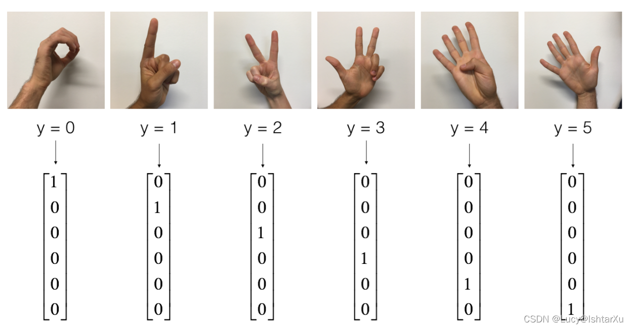

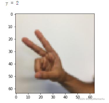
下一个单元格将向您展示数据集中带有标签的图像的示例。请随意更改下面index的值，并重新运行以查看不同的示例。

# Example of a picture
index = 6
plt.imshow(X_train_orig[index])
print ("y = " + str(np.squeeze(Y_train_orig[:, index])))

在课程2中，您已经为这个数据集构建了一个全连接网络。但由于这是一个图像数据集，因此更自然的做法是将ConvNet应用于它。

首先，让我们检查一下数据的形状。

X_train = X_train_orig/255.
X_test = X_test_orig/255.
Y_train = convert_to_one_hot(Y_train_orig, 6).T
Y_test = convert_to_one_hot(Y_test_orig, 6).T
print ("number of training examples = " + str(X_train.shape[0]))
print ("number of test examples = " + str(X_test.shape[0]))
print ("X_train shape: " + str(X_train.shape))
print ("Y_train shape: " + str(Y_train.shape))
print ("X_test shape: " + str(X_test.shape))
print ("Y_test shape: " + str(Y_test.shape))
conv_layers = {}

输出结果为

number of training examples = 1080
number of test examples = 120
X_train shape: (1080, 64, 64, 3)
Y_train shape: (1080, 6)
X_test shape: (120, 64, 64, 3)
Y_test shape: (120, 6

1.1 - 创建占位符

TensorFlow要求您为将在运行会话时输入到模型中的输入数据创建占位符。

【练习】：实现下面的函数，为输入图像$X$和输出图像$Y$创建占位符。目前不应该定义训练示例的数量。为此，您可以使用“None”作为批处理大小，它将为您提供以后选择它的灵活性。因此X的维度应该是[None, n_H0, n_W0, n_C0]， Y的维度应该是[None, n_y]。提示

# GRADED FUNCTION: create_placeholders

def create_placeholders(n_H0, n_W0, n_C0, n_y):
    """
    Creates the placeholders for the tensorflow session.
    
    Arguments:
    n_H0 -- scalar, height of an input image
    n_W0 -- scalar, width of an input image
    n_C0 -- scalar, number of channels of the input
    n_y -- scalar, number of classes
        
    Returns:
    X -- placeholder for the data input, of shape [None, n_H0, n_W0, n_C0] and dtype "float"
    Y -- placeholder for the input labels, of shape [None, n_y] and dtype "float"
    """
    
    ### START CODE HERE ### (≈2 lines)
    """
    如果这里是tf1的，直接写
    X = tf.placeholder(shape=[None, n_H0, n_W0, n_C0], dtype = "float")
    Y = tf.placeholder(shape=[None, n_y], dtype = "float")
    """
    X = tf.compat.v1.placeholder(shape=[None, n_H0, n_W0, n_C0], dtype = "float")
    Y = tf.compat.v1.placeholder(shape=[None, n_y], dtype = "float")
    ### END CODE HERE ###
    
    return X, Y

X, Y = create_placeholders(64, 64, 3, 6)
print ("X = " + str(X))
print ("Y = " + str(Y))

输出结果为

X = Tensor("Placeholder:0", shape=(?, 64, 64, 3), dtype=float32)
Y = Tensor("Placeholder_1:0", shape=(?, 6), dtype=float32)

1.2 - 初始化参数

你将使用tf.contrib.layers.xavier_initializer(seed = 0)初始化weights/filter $W1$和$W2$。你不需要担心偏差变量，因为你很快就会看到TensorFlow函数处理偏差。还请注意，您将只初始化conv2d函数的权重/过滤器。TensorFlow自动初始化全连接部分的层。我们在以后的作业中会详细讨论。
【注意】：tf2把上面那个函数取消了，经测试，tf.initializers.GlorotUniform()和上面函数效果一致

练习:实现initialize_parameters()。下面提供了每组过滤器的尺寸。提示:初始化Tensorflow中shape[1,2,3,4]的参数$W$，使用:

W = tf.get_variable("W", [1,2,3,4], initializer = ...)

# GRADED FUNCTION: initialize_parameters

def initialize_parameters():
    """
    Initializes weight parameters to build a neural network with tensorflow. The shapes are:
                        W1 : [4, 4, 3, 8]
                        W2 : [2, 2, 8, 16]
    Returns:
    parameters -- a dictionary of tensors containing W1, W2
    如果可以把tf2禁了，不需要我这么麻烦
    """
    
    tf.compat.v1.set_random_seed(1)                              # so that your "random" numbers match ours
        
    ### START CODE HERE ### (approx. 2 lines of code)
    W1 = tf.compat.v1.get_variable("W1",[4, 4, 3, 8], initializer = tf.initializers.GlorotUniform())
    W2 = tf.compat.v1.get_variable("W2",[2, 2, 8, 16], initializer =tf.initializers.GlorotUniform())
    ### END CODE HERE ###

    parameters = {"W1": W1,
                  "W2": W2}
    
    return parameters

tf.compat.v1.reset_default_graph()
with tf.compat.v1.Session() as sess_test:
    parameters = initialize_parameters()
    init = tf.compat.v1.global_variables_initializer()
    sess_test.run(init)
    print("W1 = " + str(parameters["W1"].eval()[1,1,1]))
    print("W2 = " + str(parameters["W2"].eval()[1,1,1]))

输出结果
和官方不一样…找到错误再说吧

W1 = [ 0.00131723  0.1417614  -0.04434952  0.09197326  0.14984085 -0.03514394
 -0.06847463  0.05245192]
W2 = [ 0.19037306  0.05684656  0.1125446  -0.23109215 -0.22926426  0.04337913
 -0.12032002 -0.01428771  0.04773349  0.1976018   0.0700236   0.24014717
 -0.2141701   0.09505171 -0.19955802  0.19850826]

1.3 - 前向传播

在TensorFlow中，有一些内置函数可以帮你完成卷积的步骤。

• tf.nn.conv2d(X,W1, strides = [1,s,s,1], padding = 'SAME'):给定一个输入$X$和一组过滤器𝑊1，该函数对𝑊1的过滤器$X$进行卷积。第三个输入([1,f,f,1])表示输入(m, n_H_prev, n_W_prev, n_C_prev)的每个维度的strides。你可以在这里阅读完整的文档
• tf.nn.max_pool(A, ksize = [1,f,f,1], strides = [1,s,s,1], padding = 'SAME'):给定一个输入A，这个函数使用一个大小为(f, f)的窗口和大小为(s, s)的strides来对每个窗口执行max pooling。你可以在这里阅读完整的文档
• tf.nn.relu(Z1):计算Z1的elementwise ReLU(可以是任何形状)。你可以在这里阅读完整的文档。
• tf.contrib.layers.flatten(P):给定一个输入P，该函数将每个样本扁平化为一个1D向量，同时保持批处理大小。它返回一个扁平的张量，形状为[batch_size, k]。你可以在这里阅读完整的文档。
• tf.contrib.layers.fully_connected(F, num_outputs):
  给定一个扁平的输入F，它返回使用全连接层计算得到的输出。你可以在这里阅读完整的文档。

在上面的最后一个函数tf.contrib.layers.fully_connected(F, num_outputs):中，全连接层自动初始化图中的权值，并在训练模型时继续训练它们。因此，在初始化参数时，不需要初始化这些权重。

练习:

实现下面的forward_propagation函数，构建如下模型:CONV2D -> RELU -> MAXPOOL -> CONV2D -> RELU -> MAXPOOL -> FLATTEN -> fullconnected。您应该使用上面的函数。

在细节中,我们将使用以下参数的所有步骤:
Conv2D：步长=1,填充“SAME”
ReLU - Max pool：使用一个8x8过滤器的大小和一个8×8步长,填充“SAME”Conv2D：步长=1,填充“SAME”
ReLU
Max pooling：使用一个4×4过滤器的大小和一个4×4步长,填充“SAME”
展平之前的输出
FC (full - connected)层:全连接层，无非线性激活功能。

不要在这里调用softmax。这将导致输出层中有6个神经元，然后这些神经元随后被传递到softmax。在TensorFlow中，softmax和cost函数被合并到一个单独的函数中，当计算cost时，你会调用一个不同的函数。

# GRADED FUNCTION: forward_propagation

def forward_propagation(X, parameters):
    """
    Implements the forward propagation for the model:
    CONV2D -> RELU -> MAXPOOL -> CONV2D -> RELU -> MAXPOOL -> FLATTEN -> FULLYCONNECTED

    Arguments:
    X -- input dataset placeholder, of shape (input size, number of examples)
    parameters -- python dictionary containing your parameters "W1", "W2"
                  the shapes are given in initialize_parameters

    Returns:
    Z3 -- the output of the last LINEAR unit
    以下都是tf1的代码，不改了。。。我用tf2疯狂报错，改不动了- -
    """

    # Retrieve the parameters from the dictionary "parameters" 
    W1 = parameters['W1']
    W2 = parameters['W2']
    
    ### START CODE HERE ###
    # CONV2D: stride of 1, padding 'SAME'
    Z1 = tf.nn.conv2d(X,W1, strides = [1,1,1,1], padding = 'SAME')
    # RELU
    A1 = tf.nn.relu(Z1)
    # MAXPOOL: window 8x8, sride 8, padding 'SAME'
    P1 = tf.nn.max_pool(A1, ksize = [1,8,8,1], strides = [1,8,8,1], padding = 'SAME')
    # CONV2D: filters W2, stride 1, padding 'SAME'
    Z2 = tf.nn.conv2d(P1,W2, strides = [1,1,1,1], padding = 'SAME')
    # RELU
    A2 = tf.nn.relu(Z2)
    # MAXPOOL: window 4x4, stride 4, padding 'SAME'
    P2 = tf.nn.max_pool(A2, ksize = [1,4,4,1], strides = [1,4,4,1], padding = 'SAME')
    # FLATTEN
    P2 = tf.contrib.layers.flatten(P2)
    # FULLY-CONNECTED without non-linear activation function (not not call softmax).
    # 6 neurons in output layer. Hint: one of the arguments should be "activation_fn=None"
    Z3 = tf.contrib.layers.fully_connected(P2, num_outputs = 6, activation_fn=None)
    ### END CODE HERE ###


    return Z3

tf.reset_default_graph()

with tf.Session() as sess:
    np.random.seed(1)
    X, Y = create_placeholders(64, 64, 3, 6)
    parameters = initialize_parameters()
    Z3 = forward_propagation(X, parameters)
    init = tf.global_variables_initializer()
    sess.run(init)
    a = sess.run(Z3, {X: np.random.randn(2,64,64,3), Y: np.random.randn(2,6)})
    print("Z3 = " + str(a))

输出结果为

Z3 = [[-0.44670227 -1.57208765 -1.53049231 -2.31013036 -1.29104376  0.46852064]
 [-0.17601591 -1.57972014 -1.4737016  -2.61672091 -1.00810647  0.5747785 ]]

1.4 - 计算成本

实现下面的计算成本函数。你可能会发现这两个函数很有用:

• tf.nn.softmax_cross_entropy_with_logits(logits = Z3, labels =Y):计算softmax熵损失。这个函数既计算softmax激活函数，也计算由此产生的损失。你可以在这里查看完整的文档。
• tf.reduce_mean: 计算张量各个维度元素的平均值。用这个公式把所有例子的损失加起来，得到总成本。你可以在这里查看完整的文档。

练习：使用上面的函数计算下面的成本。

# GRADED FUNCTION: compute_cost 

def compute_cost(Z3, Y):
    """
    Computes the cost
    
    Arguments:
    Z3 -- output of forward propagation (output of the last LINEAR unit), of shape (6, number of examples)
    Y -- "true" labels vector placeholder, same shape as Z3
    
    Returns:
    cost - Tensor of the cost function
    """
    
    ### START CODE HERE ### (1 line of code)
    cost = tf.reduce_mean(tf.nn.softmax_cross_entropy_with_logits(logits=Z3, labels=Y))
    ### END CODE HERE ###
    
    return cost

tf.reset_default_graph()

with tf.Session() as sess:
    np.random.seed(1)
    X, Y = create_placeholders(64, 64, 3, 6)
    parameters = initialize_parameters()
    Z3 = forward_propagation(X, parameters)
    cost = compute_cost(Z3, Y)
    init = tf.global_variables_initializer()
    sess.run(init)
    a = sess.run(cost, {X: np.random.randn(4,64,64,3), Y: np.random.randn(4,6)})
    print("cost = " + str(a))

输出

cost = 2.91034

1.5 - 模型

最后，您将合并上面实现的helper函数来构建模型。您将在SIGNS数据集上训练它。

你已经在课程2实现了random_mini_batches()。记住，这个函数返回一个小批量的列表。

练习:完成下列功能。

以下模型应该:

• 创建占位符
• 初始化参数
• 向前传播
• 计算出成本
• 创建一个优化器

最后，您将创建一个会话并为num_epochs运行一个for循环，获取小批量，然后为每个小批量优化函数。

# GRADED FUNCTION: model

def model(X_train, Y_train, X_test, Y_test, learning_rate = 0.009,
          num_epochs = 100, minibatch_size = 64, print_cost = True):
    """
    Implements a three-layer ConvNet in Tensorflow:
    CONV2D -> RELU -> MAXPOOL -> CONV2D -> RELU -> MAXPOOL -> FLATTEN -> FULLYCONNECTED
    
    Arguments:
    X_train -- training set, of shape (None, 64, 64, 3)
    Y_train -- test set, of shape (None, n_y = 6)
    X_test -- training set, of shape (None, 64, 64, 3)
    Y_test -- test set, of shape (None, n_y = 6)
    learning_rate -- learning rate of the optimization
    num_epochs -- number of epochs of the optimization loop
    minibatch_size -- size of a minibatch
    print_cost -- True to print the cost every 100 epochs
    
    Returns:
    train_accuracy -- real number, accuracy on the train set (X_train)
    test_accuracy -- real number, testing accuracy on the test set (X_test)
    parameters -- parameters learnt by the model. They can then be used to predict.
    """
    
    ops.reset_default_graph()                         # to be able to rerun the model without overwriting tf variables
    tf.set_random_seed(1)                             # to keep results consistent (tensorflow seed)
    seed = 3                                          # to keep results consistent (numpy seed)
    (m, n_H0, n_W0, n_C0) = X_train.shape             
    n_y = Y_train.shape[1]                            
    costs = []                                        # To keep track of the cost
    
    # Create Placeholders of the correct shape
    ### START CODE HERE ### (1 line)
    X, Y = create_placeholders(n_H0, n_W0, n_C0, n_y)
    ### END CODE HERE ###

    # Initialize parameters
    ### START CODE HERE ### (1 line)
    parameters = initialize_parameters()
    ### END CODE HERE ###
    
    # Forward propagation: Build the forward propagation in the tensorflow graph
    ### START CODE HERE ### (1 line)
    Z3 = forward_propagation(X, parameters)
    ### END CODE HERE ###
    
    # Cost function: Add cost function to tensorflow graph
    ### START CODE HERE ### (1 line)
    cost = compute_cost(Z3, Y)
    ### END CODE HERE ###
    
    # Backpropagation: Define the tensorflow optimizer. Use an AdamOptimizer that minimizes the cost.
    ### START CODE HERE ### (1 line)
    optimizer = tf.train.AdamOptimizer(learning_rate=learning_rate).minimize(cost)
    ### END CODE HERE ###
    
    # Initialize all the variables globally
    init = tf.global_variables_initializer()
     
    # Start the session to compute the tensorflow graph
    with tf.Session() as sess:
        
        # Run the initialization
        sess.run(init)
        
        # Do the training loop
        for epoch in range(num_epochs):

            minibatch_cost = 0.
            num_minibatches = int(m / minibatch_size) # number of minibatches of size minibatch_size in the train set
            seed = seed + 1
            minibatches = random_mini_batches(X_train, Y_train, minibatch_size, seed)

            for minibatch in minibatches:

                # Select a minibatch
                (minibatch_X, minibatch_Y) = minibatch
                # IMPORTANT: The line that runs the graph on a minibatch.
                # Run the session to execute the optimizer and the cost, the feedict should contain a minibatch for (X,Y).
                ### START CODE HERE ### (1 line)
                _ , temp_cost = sess.run([optimizer, cost], feed_dict={X:minibatch_X, Y:minibatch_Y})
                ### END CODE HERE ###
                
                minibatch_cost += temp_cost / num_minibatches
                

            # Print the cost every epoch
            if print_cost == True and epoch % 5 == 0:
                print ("Cost after epoch %i: %f" % (epoch, minibatch_cost))
            if print_cost == True and epoch % 1 == 0:
                costs.append(minibatch_cost)
        
        
        # plot the cost
        plt.plot(np.squeeze(costs))
        plt.ylabel('cost')
        plt.xlabel('iterations (per tens)')
        plt.title("Learning rate =" + str(learning_rate))
        plt.show()

        # Calculate the correct predictions
        predict_op = tf.argmax(Z3, 1)
        correct_prediction = tf.equal(predict_op, tf.argmax(Y, 1))
        
        # Calculate accuracy on the test set
        accuracy = tf.reduce_mean(tf.cast(correct_prediction, "float"))
        print(accuracy)
        train_accuracy = accuracy.eval({X: X_train, Y: Y_train})
        test_accuracy = accuracy.eval({X: X_test, Y: Y_test})
        print("Train Accuracy:", train_accuracy)
        print("Test Accuracy:", test_accuracy)
                
        return train_accuracy, test_accuracy, parameters

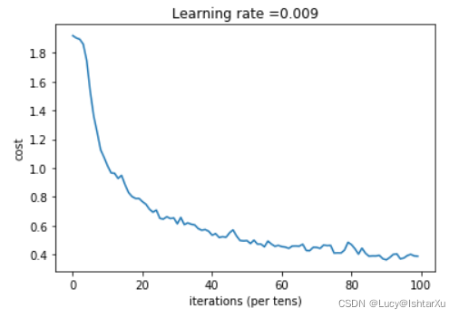
_, _, parameters = model(X_train, Y_train, X_test, Y_test)

输出结果为

Cost after epoch 0: 1.917920
Cost after epoch 5: 1.532475
Cost after epoch 10: 1.014804
Cost after epoch 15: 0.885137
Cost after epoch 20: 0.766963
Cost after epoch 25: 0.651208
Cost after epoch 30: 0.613356
Cost after epoch 35: 0.605931
Cost after epoch 40: 0.534713
Cost after epoch 45: 0.551402
Cost after epoch 50: 0.496976
Cost after epoch 55: 0.454438
Cost after epoch 60: 0.455496
Cost after epoch 65: 0.458359
Cost after epoch 70: 0.450040
Cost after epoch 75: 0.410687
Cost after epoch 80: 0.469005
Cost after epoch 85: 0.389253
Cost after epoch 90: 0.363808
Cost after epoch 95: 0.376132

Tensor(“Mean_1:0”, shape=(), dtype=float32)

恭喜你!您已经完成了作业，并建立了一个模型，识别手语的准确性接近80%的测试集。如果您愿意，可以自由地进一步使用这个数据集。实际上，您可以通过花更多的时间调整超参数或使用正则化(因为该模型显然具有很高的方差)来提高其准确性。

再一次，为你的工作竖起大拇指!

fname = "images/thumbs_up.jpg"
image = np.array(ndimage.imread(fname, flatten=False))
my_image = scipy.misc.imresize(image, size=(64,64))
plt.imshow(my_image)