参考这一篇，更容易理解

Understanding and Coding the Self-Attention Mechanism of Large Language Models From Scratch (sebastianraschka.com)

一  Self Attention 动画演示

Step 1: Prepare inputs

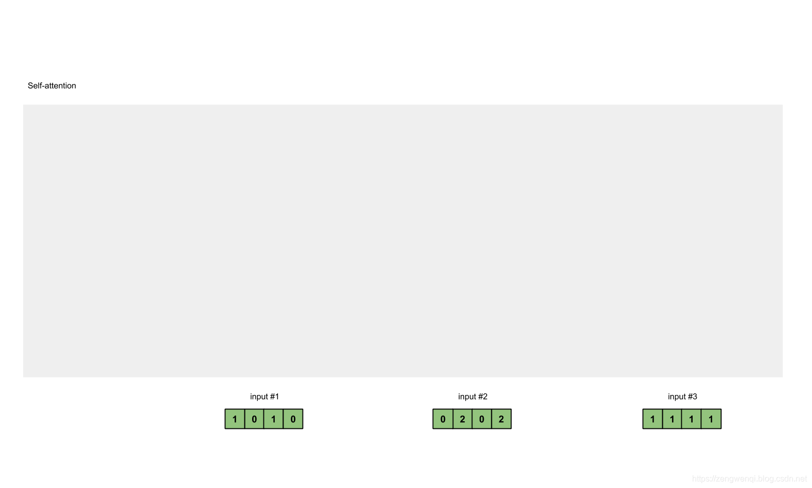
For this tutorial, we start with 3 inputs, each with dimension 4.

Input 1: [1, 0, 1, 0] 
Input 2: [0, 2, 0, 2]
Input 3: [1, 1, 1, 1]

Step 2: Initialise weights

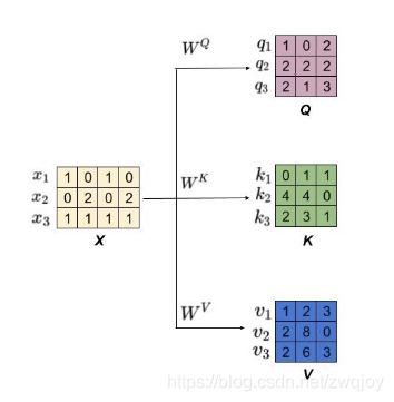
Every input must have three representations (see diagram below). These representations are called key (orange), query (red), and value (purple). For this example, let’s take that we want these representations to have a dimension of 3. Because every input has a dimension of 4, this means each set of the weights must have a shape of 4×3.

(the dimension of value is also the dimension of the output.)

In order to obtain these representations, every input (green) is multiplied with a set of weights for keys, a set of weights for querys (I know that’s not the right spelling), and a set of weights for values. In our example, we ‘initialise’ the three sets of weights as follows.

Weights for key:

[[0, 0, 1],
 [1, 1, 0],
 [0, 1, 0],
 [1, 1, 0]]

Weights for query:

[[1, 0, 1],
 [1, 0, 0],
 [0, 0, 1],
 [0, 1, 1]]

Weights for value:

[[0, 2, 0],
 [0, 3, 0],
 [1, 0, 3],
 [1, 1, 0]]

PS： In a neural network setting, these weights are usually small numbers, initialised randomly using an appropriate random distribution like Gaussian, Xavier and Kaiming distributions.

Step 3: Derive key, query and value

Now that we have the three sets of weights, let’s actually obtain the key, query and value representations for every input.

Key representation for Input 1:

               [0, 0, 1]
[1, 0, 1, 0] x [1, 1, 0] = [0, 1, 1]
               [0, 1, 0]
               [1, 1, 0]

Use the same set of weights to get the key representation for Input 2:

               [0, 0, 1]
[0, 2, 0, 2] x [1, 1, 0] = [4, 4, 0]
               [0, 1, 0]
               [1, 1, 0]

Use the same set of weights to get the key representation for Input 3:

               [0, 0, 1]
[1, 1, 1, 1] x [1, 1, 0] = [2, 3, 1]
               [0, 1, 0]
               [1, 1, 0]

1.   A faster way is to vectorise the above key operations:

               [0, 0, 1]
[1, 0, 1, 0]   [1, 1, 0]   [0, 1, 1]
[0, 2, 0, 2] x [0, 1, 0] = [4, 4, 0]
[1, 1, 1, 1]   [1, 1, 0]   [2, 3, 1]

2.   Let’s do the same to obtain the value representations for every input:

               [0, 2, 0]
[1, 0, 1, 0]   [0, 3, 0]   [1, 2, 3] 
[0, 2, 0, 2] x [1, 0, 3] = [2, 8, 0]
[1, 1, 1, 1]   [1, 1, 0]   [2, 6, 3]

3. finally the query representations:

               [1, 0, 1]
[1, 0, 1, 0]   [1, 0, 0]   [1, 0, 2]
[0, 2, 0, 2] x [0, 0, 1] = [2, 2, 2]
[1, 1, 1, 1]   [0, 1, 1]   [2, 1, 3]

PS: In practice, a bias vector may be added to the product of matrix multiplication.

Step 4: Calculate attention scores for Input 1

To obtain attention scores, we start off with taking a dot product between Input 1’s query (red) with all keys (orange), including itself. Since there are 3 key representations (because we have 3 inputs), we obtain 3 attention scores (blue).

            [0, 4, 2]
[1, 0, 2] x [1, 4, 3] = [2, 4, 4]
            [1, 0, 1]

we only use the query from Input 1. Later we’ll work on repeating this same step for the other querys.

PS: The above operation is known as dot product attention, one of the several score functions. Other score functions include scaled dot product and additive/concat.

Step 5: Calculate softmax

Take the softmax across these attention scores (blue).

softmax([2, 4, 4]) = [0.0, 0.5, 0.5]

Step 6: Multiply scores with values

The softmaxed attention scores for each input (blue) is multiplied with its corresponding value (purple). This results in 3 alignment vectors (yellow). In this tutorial, we’ll refer to them as weighted values.

1: 0.0 * [1, 2, 3] = [0.0, 0.0, 0.0]
2: 0.5 * [2, 8, 0] = [1.0, 4.0, 0.0]
3: 0.5 * [2, 6, 3] = [1.0, 3.0, 1.5]

Step 7: Sum weighted values to get Output 1

Take all the weighted values (yellow) and sum them element-wise:

  [0.0, 0.0, 0.0]
+ [1.0, 4.0, 0.0]
+ [1.0, 3.0, 1.5]
-----------------
= [2.0, 7.0, 1.5]

The resulting vector [2.0, 7.0, 1.5] (dark green) is Output 1, which is based on the query representation from Input 1 interacting with all other keys, including itself.

Step 8: Repeat for Input 2 & Input 3

Query 与 Key 的纬度一定要相同，因为两者需要进行点积相乘， 然而， Value的纬度可以与Q, K的纬度不一样

The resulting output will consequently follow the dimension of value.

二  Self-Attention代码演示

Step 1: 准备输入X

import tensorflow as tf

x = [
  [1, 0, 1, 0], # Input 1
  [0, 2, 0, 2], # Input 2
  [1, 1, 1, 1]  # Input 3
 ]
x = tf.Variable(x, dtype=tf.float32)

Step 2: 参数W初始化

一般使用_Gaussian, Xavier_ 和 _Kaiming_随机分布初始化。在训练开始之前完成这些初始化工作。

w_key = [
  [0, 0, 1],
  [1, 1, 0],
  [0, 1, 0],
  [1, 1, 0]
]
w_query = [
  [1, 0, 1],
  [1, 0, 0],
  [0, 0, 1],
  [0, 1, 1]
]
w_value = [
  [0, 2, 0],
  [0, 3, 0],
  [1, 0, 3],
  [1, 1, 0]
]


w_key = tf.Variable(w_key, dtype=tf.float32)
w_query = tf.Variable(w_query, dtype=tf.float32)
w_value = tf.Variable(w_value, dtype=tf.float32)

Step 3:并计算出K, Q, V

    

keys = x @ w_key
querys = x @ w_query
values = x @ w_value

print(keys)
# tensor([[0., 1., 1.],
#         [4., 4., 0.],
#         [2., 3., 1.]])

print(querys)
# tensor([[1., 0., 2.],
#         [2., 2., 2.],
#         [2., 1., 3.]])

print(values)
# tensor([[1., 2., 3.],
#         [2., 8., 0.],
#         [2., 6., 3.]])

Step 4: 计算注意力权重

首先计算注意力权重，通过计算K的转置矩阵和Q的点积得到。

attn_scores = querys @ tf.transpose(keys, perm=[1, 0])  # [[1, 4]
print(attn_scores)
# tensor([[ 2.,  4.,  4.],  # attention scores from Query 1
#         [ 4., 16., 12.],  # attention scores from Query 2
#         [ 4., 12., 10.]]) # attention scores from Query 3

Step 5: 计算 softmax

例子中没有去除   

attn_scores_softmax = tf.nn.softmax(attn_scores)
print(attn_scores_softmax)
# tensor([[6.3379e-02, 4.6831e-01, 4.6831e-01],
#         [6.0337e-06, 9.8201e-01, 1.7986e-02],
#         [2.9539e-04, 8.8054e-01, 1.1917e-01]])

# For readability, approximate the above as follows
attn_scores_softmax = [
  [0.0, 0.5, 0.5],
  [0.0, 1.0, 0.0],
  [0.0, 0.9, 0.1]
]
attn_scores_softmax = tf.Variable(attn_scores_softmax)
print(attn_scores_softmax)

下面例子除   

​​

attn_scores = attn_scores / 1.7
print(attn_scores)
attn_scores = [
    [1.2, 2.4, 2.4],
    [2.4, 9.4, 7.1],
    [2.4, 7.1, 5.9],
]
attn_scores = tf.Variable(attn_scores, dtype=tf.float32)
print(attn_scores)

attn_scores_softmax = tf.nn.softmax(attn_scores)
print(attn_scores_softmax)
attn_scores_softmax = [
    [0.1, 0.4, 0.4],
    [0.0, 0.9, 0.0],
    [0.0, 0.7, 0.2],
]
attn_scores_softmax = tf.Variable(attn_scores_softmax, dtype=tf.float32)
print(attn_scores_softmax)

​

Step6+Step7一起算出来

print(attn_scores_softmax)
print(values)
outputs = tf.matmul(attn_scores_softmax, values)
print(outputs)

<tf.Variable 'Variable:0' shape=(3, 3) dtype=float32, numpy=
array([[0. , 0.5, 0.5],
       [0. , 1. , 0. ],
       [0. , 0.9, 0.1]], dtype=float32)>
tf.Tensor(
[[1. 2. 3.]
 [2. 8. 0.]
 [2. 6. 3.]], shape=(3, 3), dtype=float32)
tf.Tensor(
[[2.        7.        1.5      ]
 [2.        8.        0.       ]
 [2.        7.7999997 0.3      ]], shape=(3, 3), dtype=float32)

下面例子使用的除   后，算出来的outputs

​​

​

Step 6: Multiply scores with values

weighted_values = values[:,None] * tf.transpose(attn_scores_softmax, perm=[1, 0])[:,:,None]
print(weighted_values)
# tensor([[[0.0000, 0.0000, 0.0000],
#          [0.0000, 0.0000, 0.0000],
#          [0.0000, 0.0000, 0.0000]],
# 
#         [[1.0000, 4.0000, 0.0000],
#          [2.0000, 8.0000, 0.0000],
#          [1.8000, 7.2000, 0.0000]],
# 
#         [[1.0000, 3.0000, 1.5000],
#          [0.0000, 0.0000, 0.0000],
#          [0.2000, 0.6000, 0.3000]]])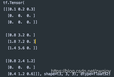

Step 7: Sum weighted values

outputs = tf.reduce_sum(weighted_values, axis=0)
print(outputs)
# tensor([[2.0000, 7.0000, 1.5000],  # Output 1
#         [2.0000, 8.0000, 0.0000],  # Output 2
#         [2.0000, 7.8000, 0.3000]]) # Output 3